Input: whole slide — one H&E patch embedding per 55 µm bin (112 µm crop at 0.5 µm/px)
Output: expression of 1,622 genes per bin
Truth: Xenium transcripts binned at 55 µm, log1p counts
Metric: per-gene PCC across a slide's bins — higher is better; mean and top-50 over genes, then mean over slides
model
ReST
Recursive model over the whole slide. Trained on public 10x slides and on BEAT patients other than the ones tested.
Checkpoint: epoch 49 (MSE), then 1 epoch with a per-gene PCC loss and a coverage-weighted PCC on rare genes; depth 4. “ReST ep29” = the earlier MSE-only checkpoint.
evaluation sets
set (click a row for organs / disease)
slides
ReST trained on this cohort?
BEAT mesothelioma, held-out patients
108
yes, other patients
10x / HEST test fold
18
yes, other slides
liver, held-out donor
1
yes, other donors
unused HEST slides
29
no
old 10x slides
3
no
heart biopsy cores
195
no
ReST on every test setup
* ReST was trained on other patients / slides of these cohorts.
BEAT mesothelioma: 108 held-out patients
0.75
median gene PCC
83%
gene–slide pairs with PCC ≥ 0.5
0.65
mean gene PCC per slide
Share of gene–slide pairs (expressed genes) at or above each PCC.
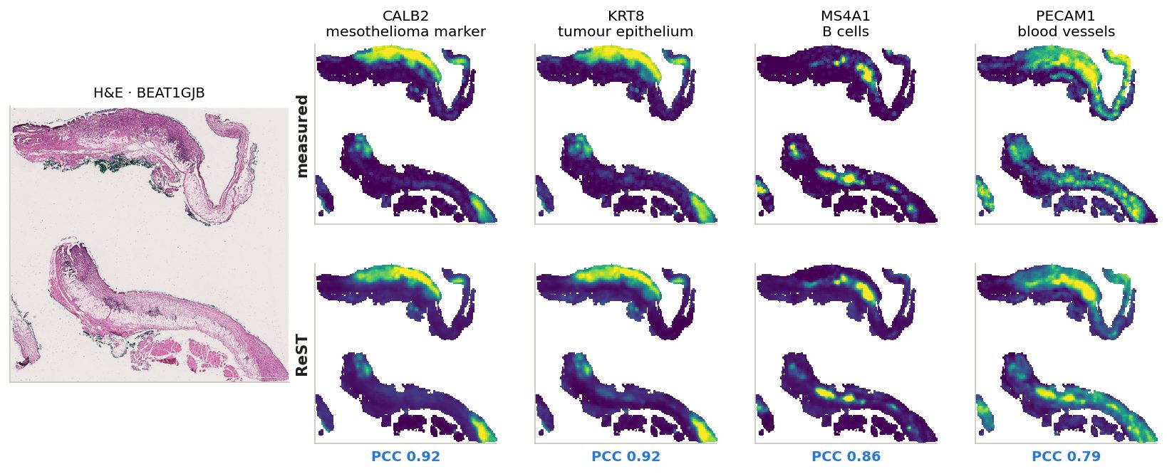
One BEAT slide, four cell types
Each map scaled to its own 2nd–98th percentile; PCC across the slide's bins.
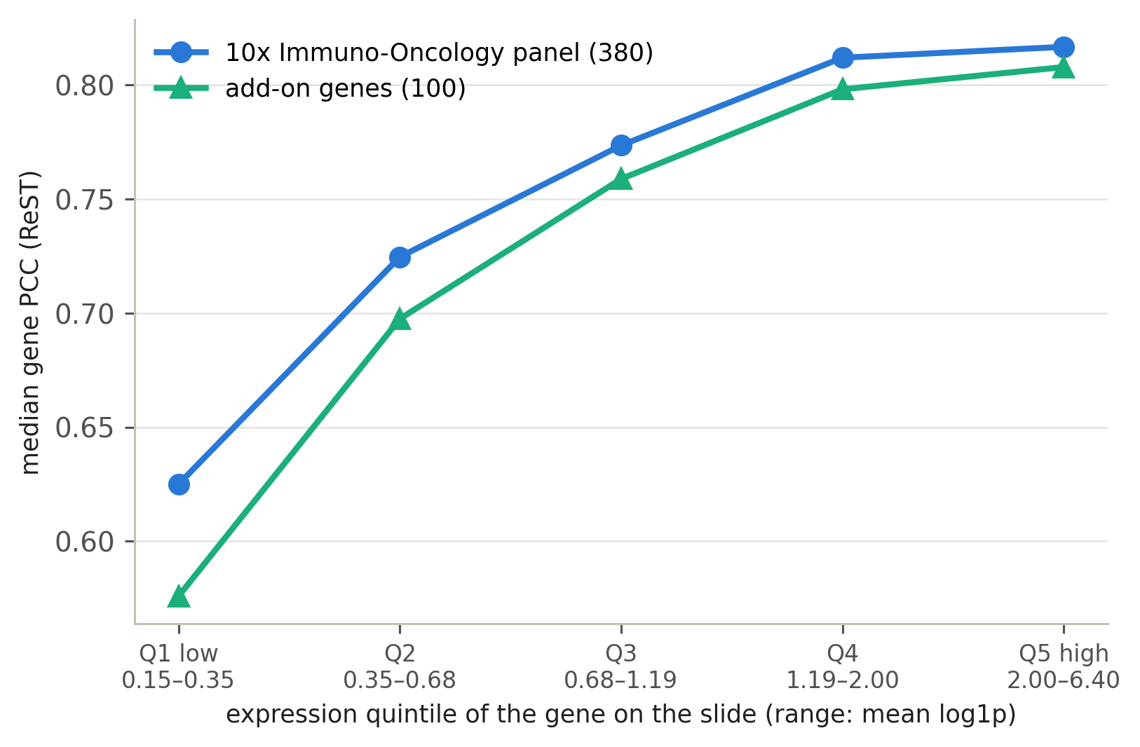
Standard 10x Immuno-Oncology panel (380) + add-on (100)
BEAT measures 480 genes: the standard 10x Xenium Human Immuno-Oncology v1 panel (380) + 100 add-on genes picked for mesothelioma
Median gene PCC within expression quintiles; add-on genes are more highly expressed on average.
expressed genes
median PCC
10x panel (369)
0.75
add-on (100)
0.75
Within quintiles the two groups are +0.01 to +0.05 PCC apart.
expression quintiles
Every gene on every slide where it is expressed (mean log1p ≥ 0.15; 41,011 gene–slide pairs) is ranked by its mean expression on that slide and cut into 5 equal groups: Q1 = the lowest 20% … Q5 = the highest 20% (ranges under the axis).
Within each group: median PCC of the 10x-panel genes and of the add-on genes. Comparing inside a group removes the effect of expression level — add-on genes are more highly expressed, and PCC rises with expression.
Gene explorer: BEAT and SPLIT
471 BEAT and 1054 SPLIT genes: each gene's 5 best and 5 worst slides, measured vs ReST vs patch MLP. Colour: Hallmark group or UniProt protein class
Cohort· organColour by
Gene explorer (FRM): BEAT and SPLIT
480 BEAT and 1054 SPLIT genes: each gene's 5 best and 5 worst slides by FRM, measured vs FRM vs ReST vs patch MLP. BEAT, expressed slides: FRM ahead of ReST on 67% and of the MLP on 92% of (slide, gene) pairs
Cohort· organ
FRM: the Fixed-Point Forcing checkpoint, t = 0 read-out. All three models on the same bins and measured genes; smoothed truth. Best / worst among the slides where the gene is expressed (mean log1p ≥ 0.15).
Gene categories: the workbook
Every BEAT and SPLIT gene: the deck's Hallmark-based category next to the protein's UniProt class, for review
Cohort: BEAT (IO) = BEAT gene on the 10x Xenium Immuno-Oncology panel; BEAT (add-on) = one of BEAT's custom add-on genes; SPLIT = measured in the SPLIT breast / lung samples.
Deck category: the most common group among the gene's Hallmark pathways (group in brackets). UniProt class: from the protein's curated UniProt keywords; basis = the keyword that decided it.
Click a header to sort; hover a gene for its UniProt function summary. Corrections go in the .xlsx (corrected_category, notes); it also has the per-gene scores and all keywords.
One row of the Genes sheet, field by field
gene
KRT5 · keratin 5
cohort
BEAT (add-on) + SPLIT
Hallmark pathways [group]
KRAS Signaling Dn [Signalling]
1
category votes
Signalling 1
2
deck category
Signalling
2
UniProt location keywords
Cytoplasm; Intermediate filament; Keratin
3
protein class (UniProt rule)
Structural: cytoskeleton
3
rule hit
location: Intermediate filament, Keratin
4
corrected_category
(empty: yours to fill)
5
1
Hallmark sets. KRT5 is a member of 1 MSigDB Hallmark set: KRAS Signaling Dn, genes that go down when KRAS signalling is on. Each set belongs to one group (sheet “Hallmark groups”).
2
Deck category = the group with most votes (one vote per set). KRT5 gets Signalling only because of that one set. When two groups tie, the “tie” column says yes and the pick between them was arbitrary.
3
Protein class comes from the protein’s own curated UniProt keywords (function, process, location), not from co-expression.
4
Rule hit = the keyword that decided it: the first matching rule in “UniProt class rules”. Here: Intermediate filament, Keratin, so a structural protein, not a signalling one.
5
Your fix goes in this column of the .xlsx. The category-score slide uses it on the next rebuild; re-exporting keeps it.
Gene categories used in the BEAT deck (gene explorer colours; scores by category).
deck category: the most common process group among the gene's MSigDB Hallmark gene sets (sheet 'Hallmark groups'). Hallmark sets are expression programmes (genes that change together in a process), not protein function: a structural protein can sit in a signalling set because it responds to that signal. 'category votes' shows the count per group; 'tie' = yes means two groups had the same count and the choice between them was arbitrary.
protein class (UniProt rule): from the protein's curated UniProt keywords, by the ordered rules in sheet 'class rules' (first match wins; 'rule hit' names the keyword). A suggestion to compare against, not ground truth.
corrected_category / notes: fill in. Any label works; category_scores.py uses corrected_category where filled, the deck category elsewhere. Re-exporting keeps these columns.
Scores: median over slides where the gene is measured and expressed (mean log1p >= 0.15), PCC across bins vs the smoothed truth; ReST (the fine-tuned model of the deck) and the patch MLP; 'ReST - MLP' = median of the per-slide difference; 'ReST ahead' = share of those slides where ReST's PCC is higher. other Xenium = 10x test fold + unused HEST + old 10x.
training slides: training slides (of 68) that measure the gene. BEAT: bins detected = median share of bins with >= 1 count.
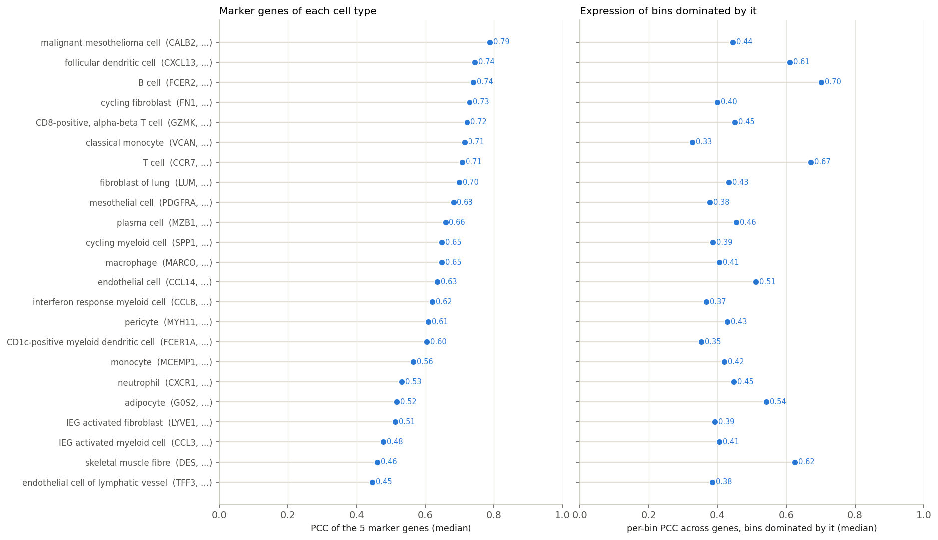
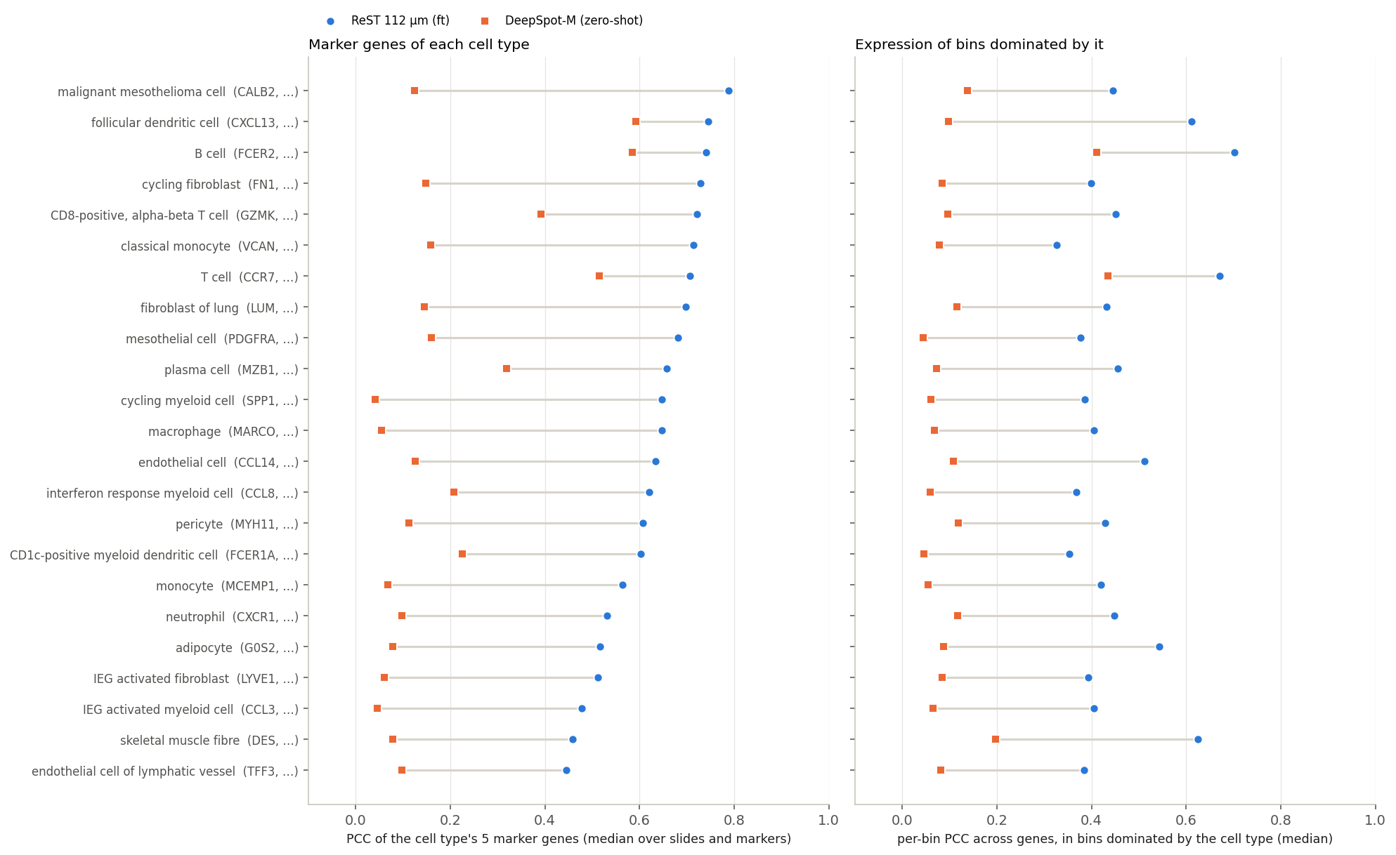
Markers: each cell type's 5 genes highest in the bins it dominates (≥ 50% of a bin's cells). Best: malignant mesothelioma cell (0.79); lowest: endothelial cell of lymphatic vessel (0.45)
Left: median PCC of each cell type's 5 marker genes. Right: PCC across genes of predicted vs true profile, in bins the cell type dominates.
Pathways: how they are scored
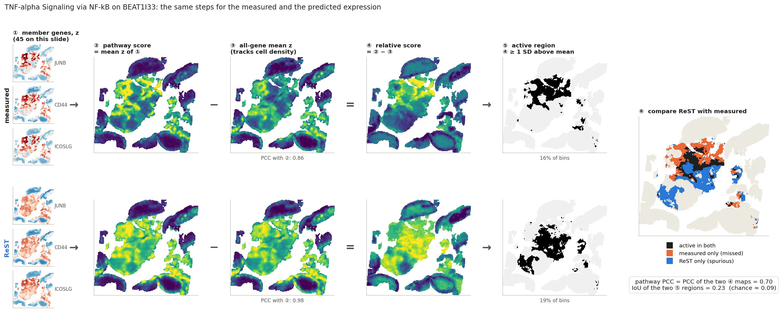
Same steps on the measured and on the predicted expression, then compare
pathways
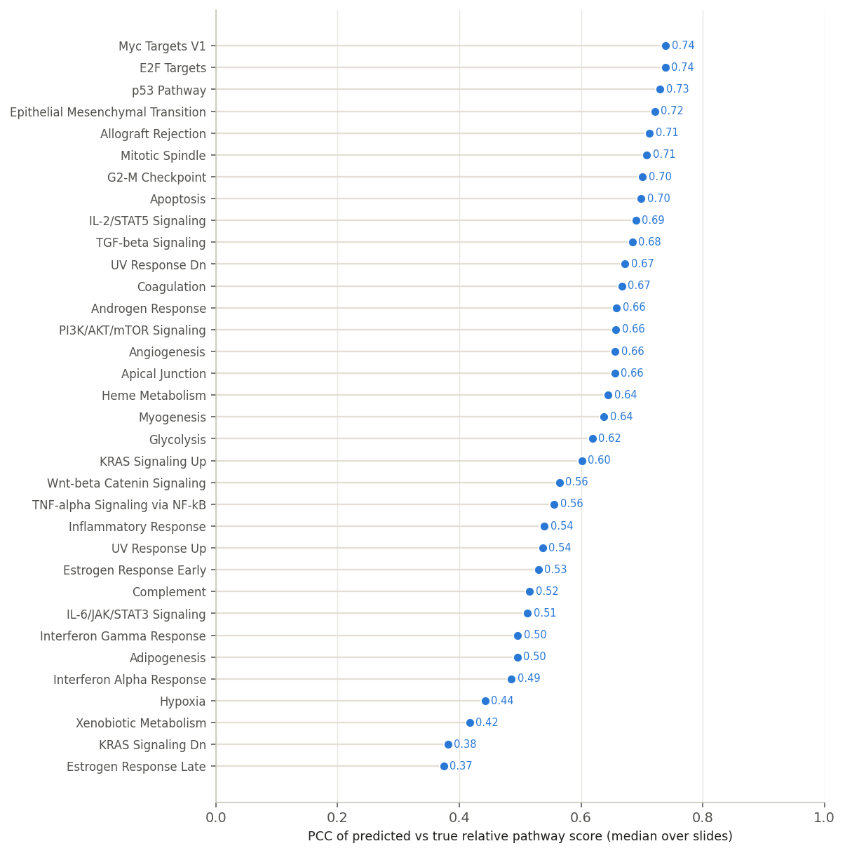
MSigDB Hallmark. Per slide: members on the panel and expressed (≥ 5). 34 pathways scored on ≥ 5 slides.
why subtract ③
Most genes rise with cell density: the raw score ② of a typical pathway correlates 0.96 with ③. ④ keeps what is specific to the pathway.
two metrics, higher is better
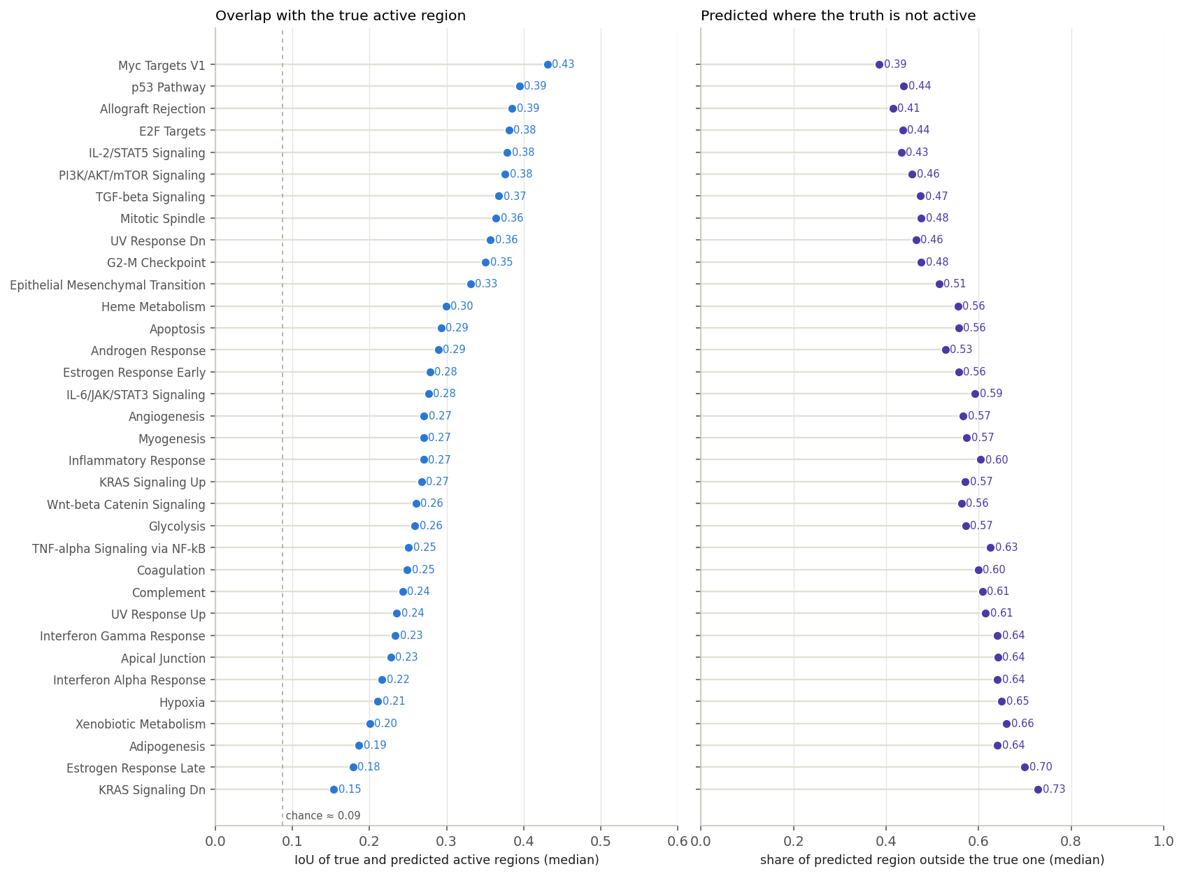
Pathway PCC: ④ predicted vs ④ measured. IoU: overlap of the two ⑤ regions; chance ≈ 0.09.
Active region = bins with relative score ≥ 1 SD above the slide mean (~16% of bins), for the truth and for the prediction
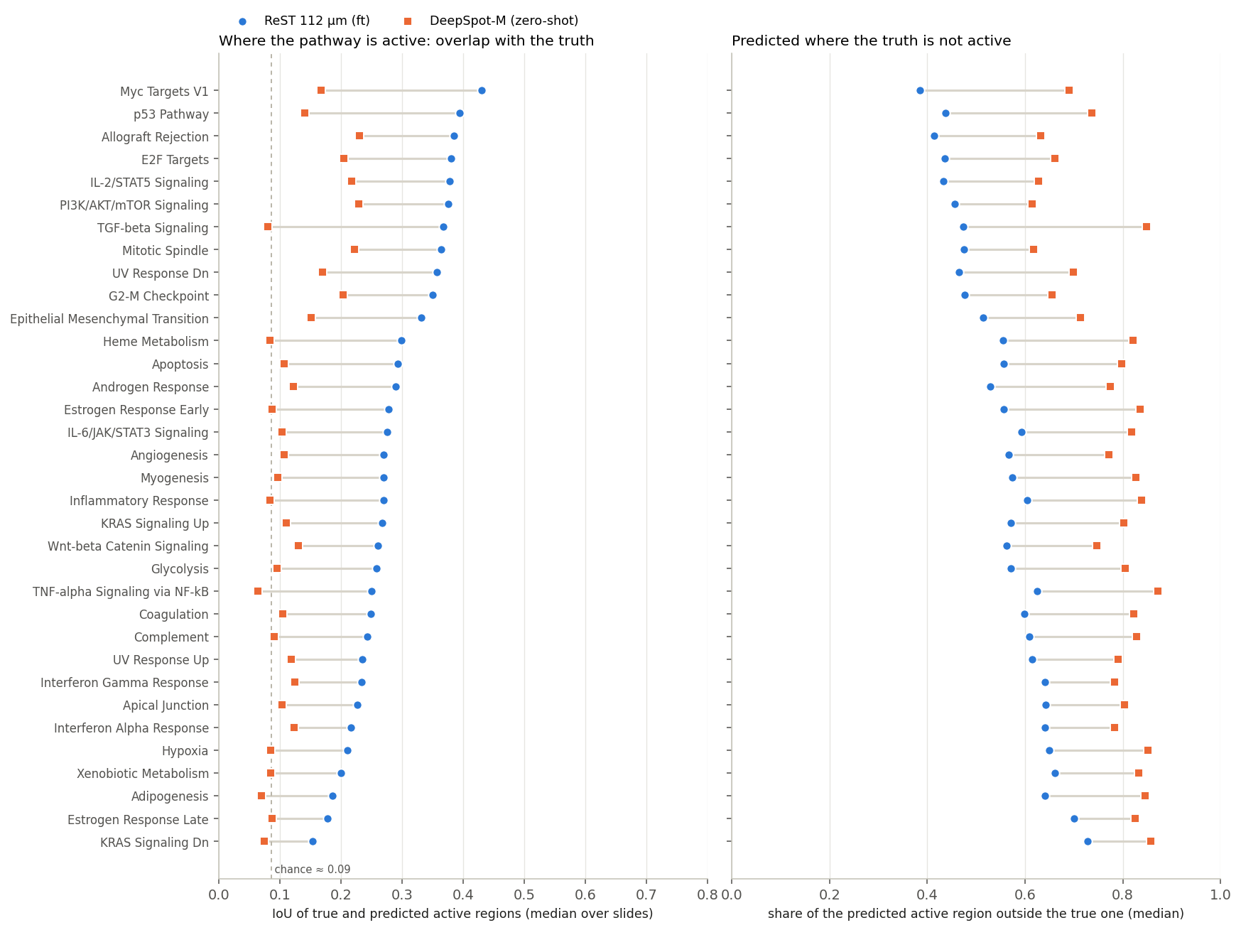
Left: IoU of true and predicted active regions (higher is better; dashed: chance). Right: share of the predicted region where the truth is not active (lower is better).
0.27
median IoU · chance: 0.09
Best placed: Myc Targets V1, p53 Pathway, Allograft Rejection, E2F Targets. Most missed, and most often predicted elsewhere: KRAS Signaling Dn, Estrogen Response Late, Adipogenesis, Xenobiotic Metabolism.
Both regions have about the same size, so missed and spurious mirror each other.
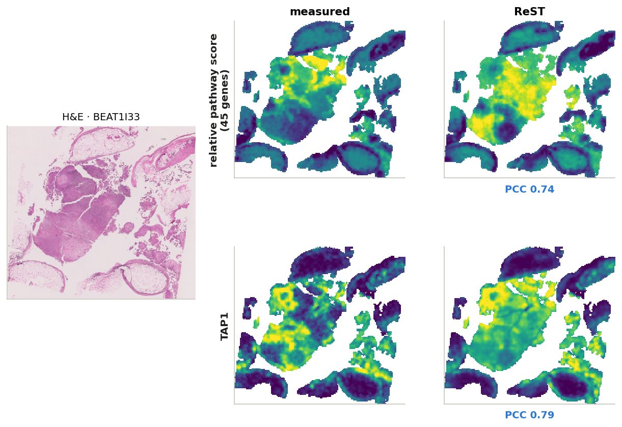
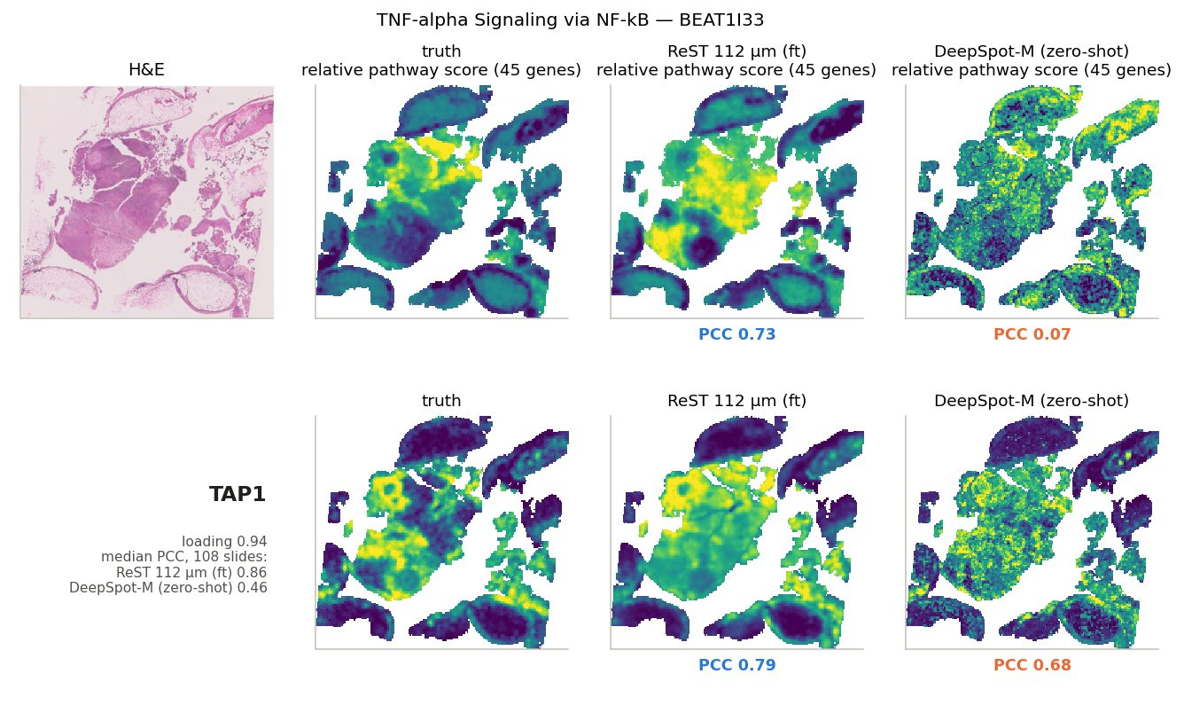
Pathway example: TNF-α signalling via NF-κB
Relative score and its most typical gene (TAP1), on the slide where the true score is most spatially structured
Median over 108 slides: 0.56.
Niches: what they are
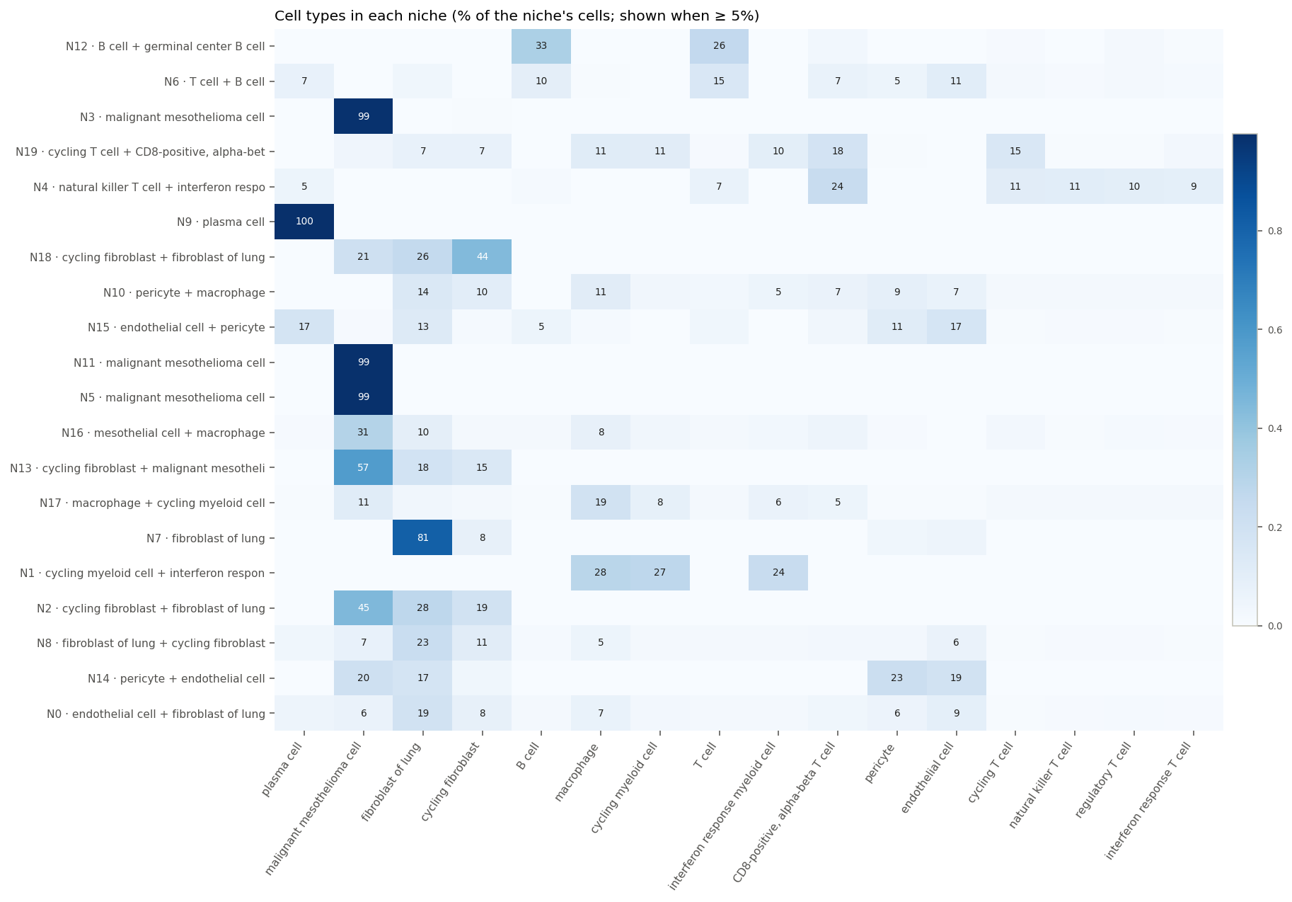
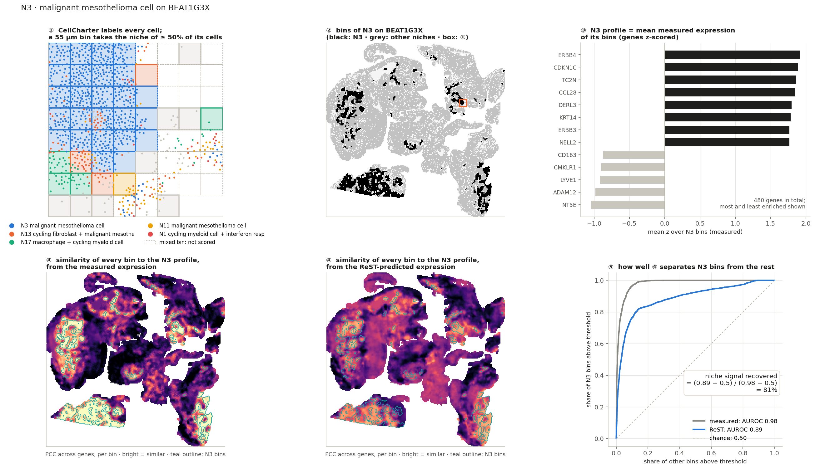
CellCharter, K = 20
Each cell is described by its own expression plus its neighbours' (5 hops, 20 µm graph)
Cells are clustered into 20 niche types across all BEAT samples
A bin takes the niche of most of its cells (≥ 50% agree)
Names: cell types most enriched in the niche
1,018,637 bins with a clear niche on 103 slides. ReST never saw these labels.
groups by H&E visibility (team)
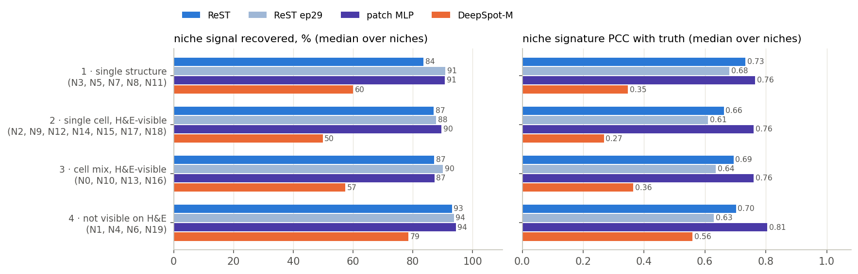
1 · single structure
tumour or stroma sheets
N3, N5, N7, N8, N11
2 · single cell
one H&E-visible cell type: plasma, B / germinal centre, vessel, macrophage, cycling fibroblast
N2, N9, N12, N14, N15, N17, N18
3 · cell mix
H&E-visible cell combinations
N0, N10, N13, N16
4 · the rest
immune cell states: interferon response, cycling, cytotoxic, T + B aggregates
N1, N4, N6, N19
Groups 1–3 a pathologist can call from H&E; group 4 needs expression. Hover a row for the niche names.
Share of each niche's cells by cell type.
Niches: how they are scored
Centroids come from the measured data; ReST never saw niche labels
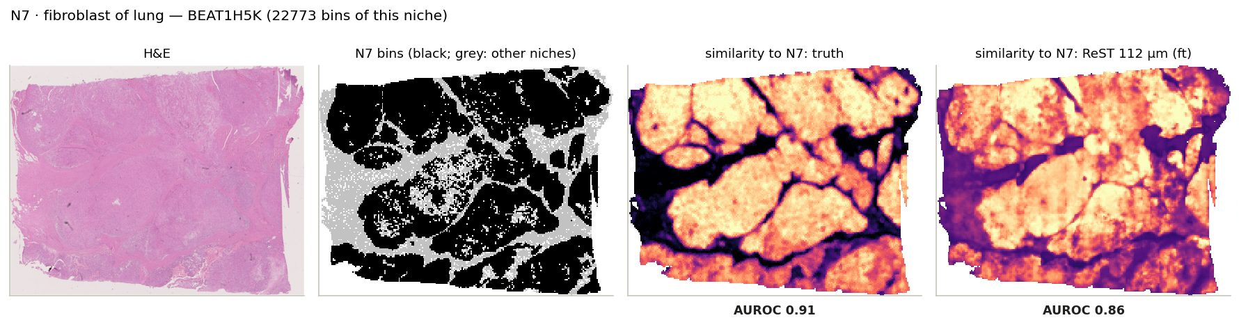
niche signal recovered $= \dfrac{\mathrm{AUROC}_{\mathrm{ReST}}-0.5}{\mathrm{AUROC}_{\mathrm{measured}}-0.5}$
· 0% = chance, 100% = separates the niche as well as the measured expression · per slide, per niche with ≥ 30 bins
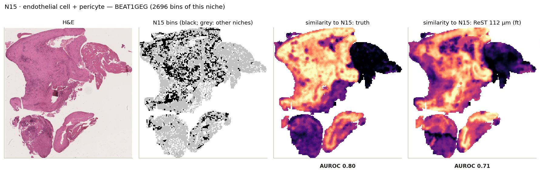
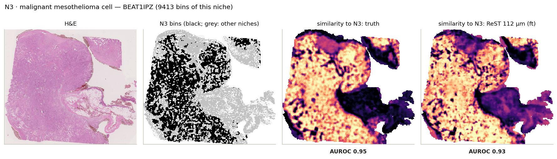
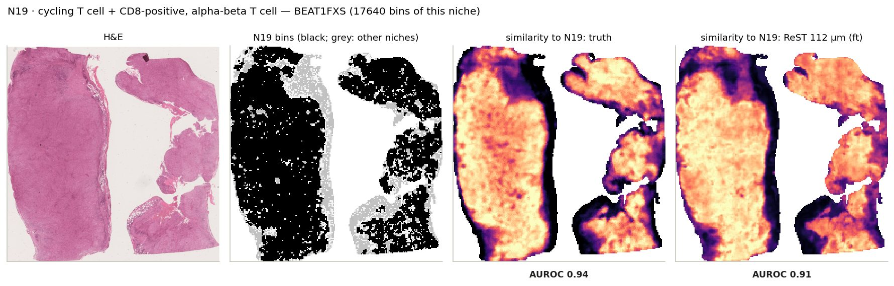
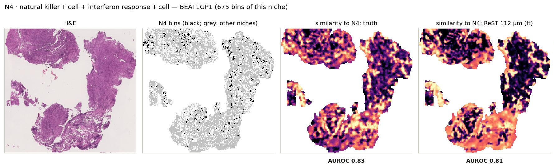
Niche similarity maps, niche by niche
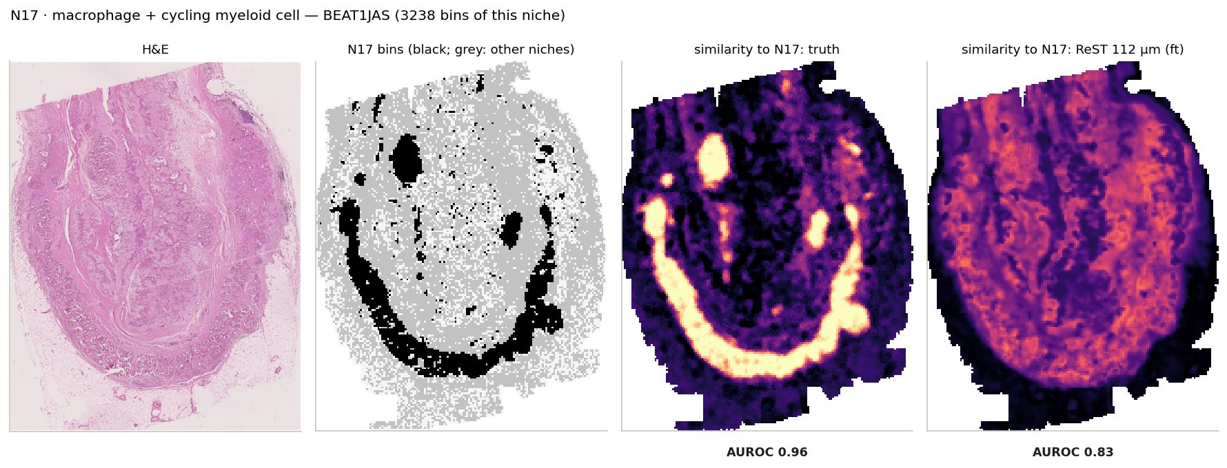
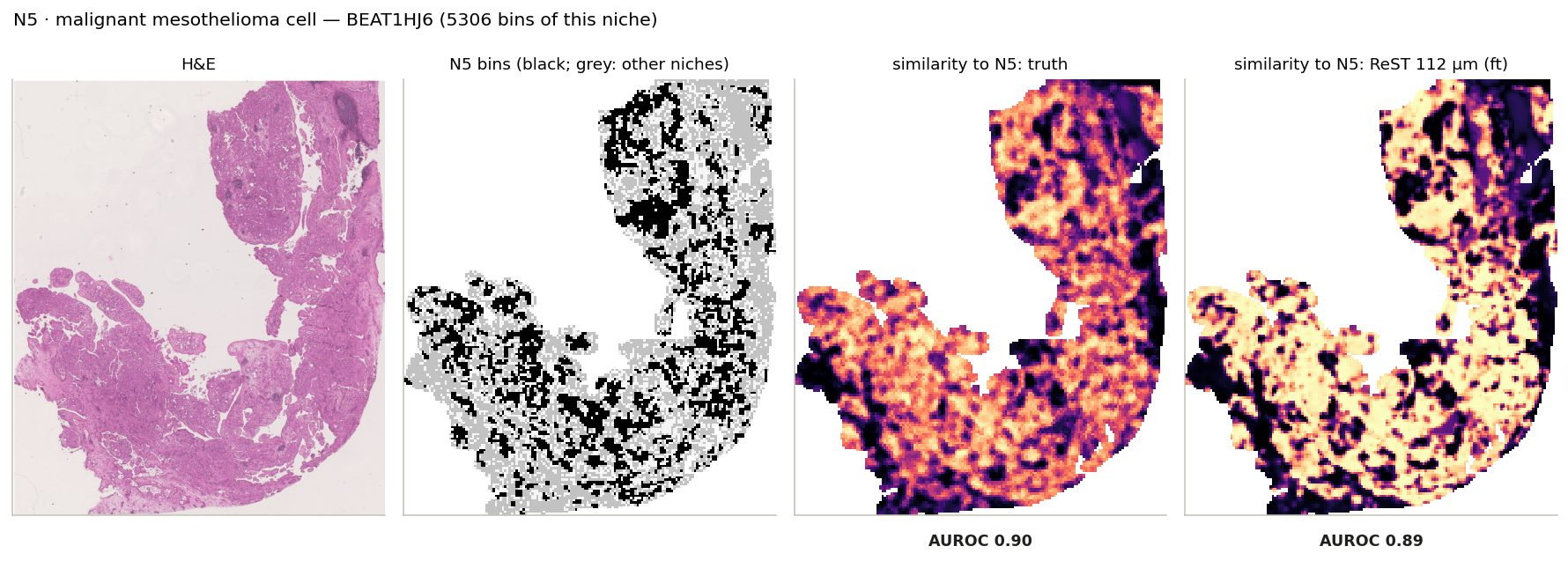
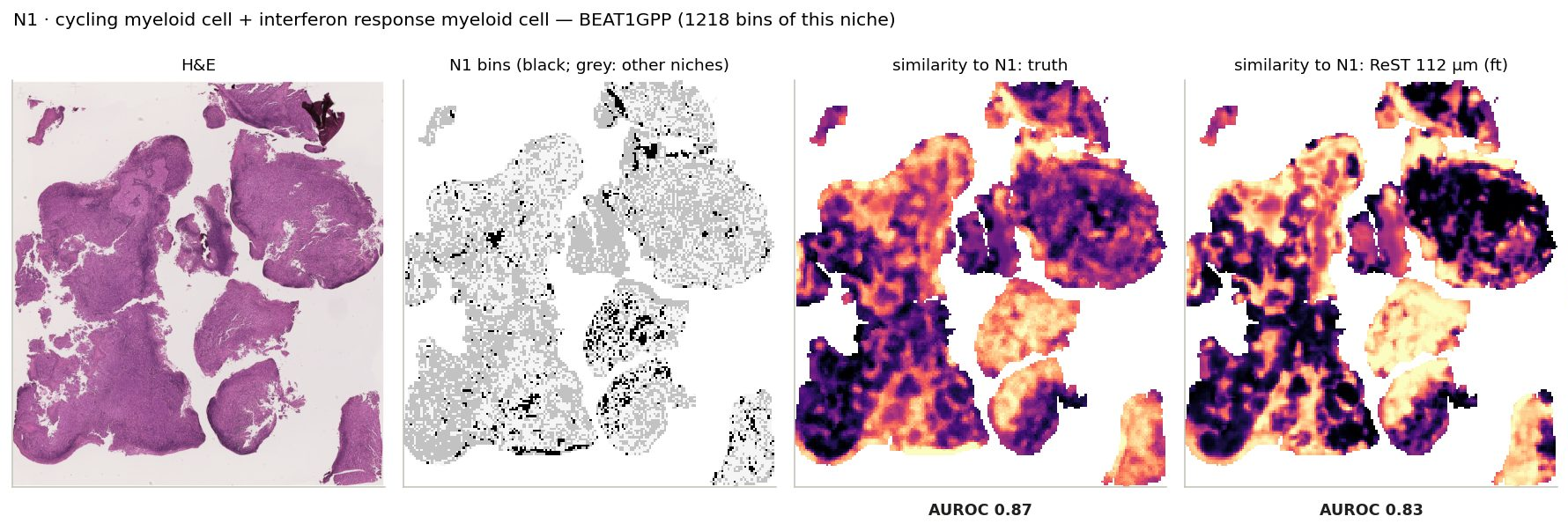
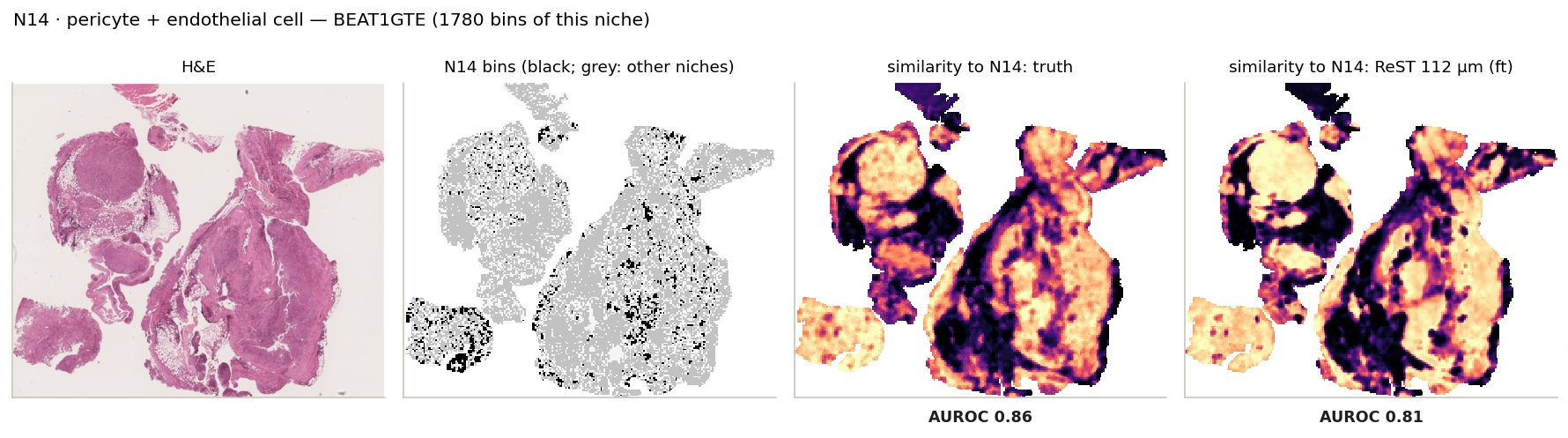
Click a niche: its bins on the slide where it is largest, and the similarity maps from the measured and the ReST-predicted expression
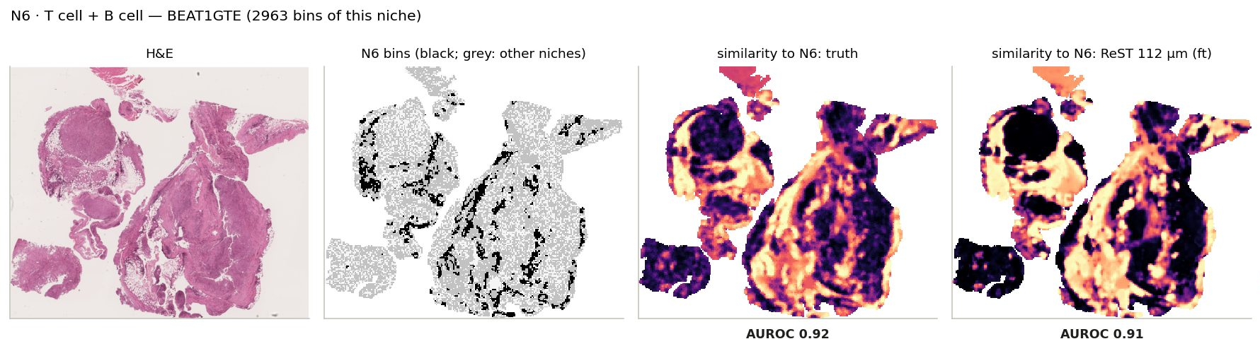
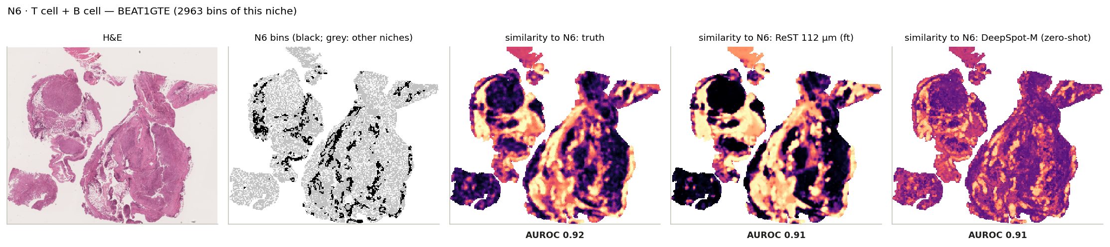
N6 · T cell + B cell: its bins on the slide where it is largest, and every bin's similarity to its centroid from the truth and from ReST.
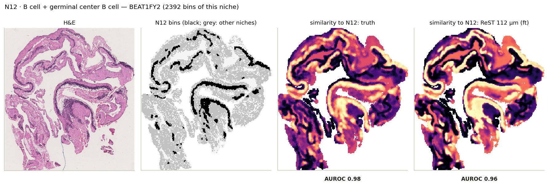
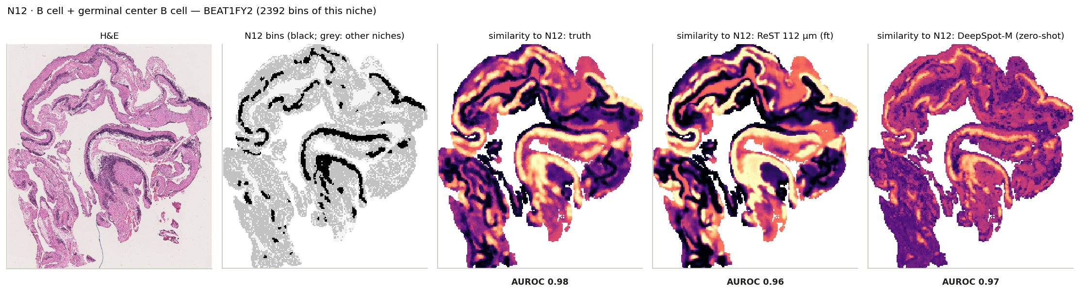
N12 · B cell + germinal center B cell: its bins on the slide where it is largest, and every bin's similarity to its centroid from the truth and from ReST.
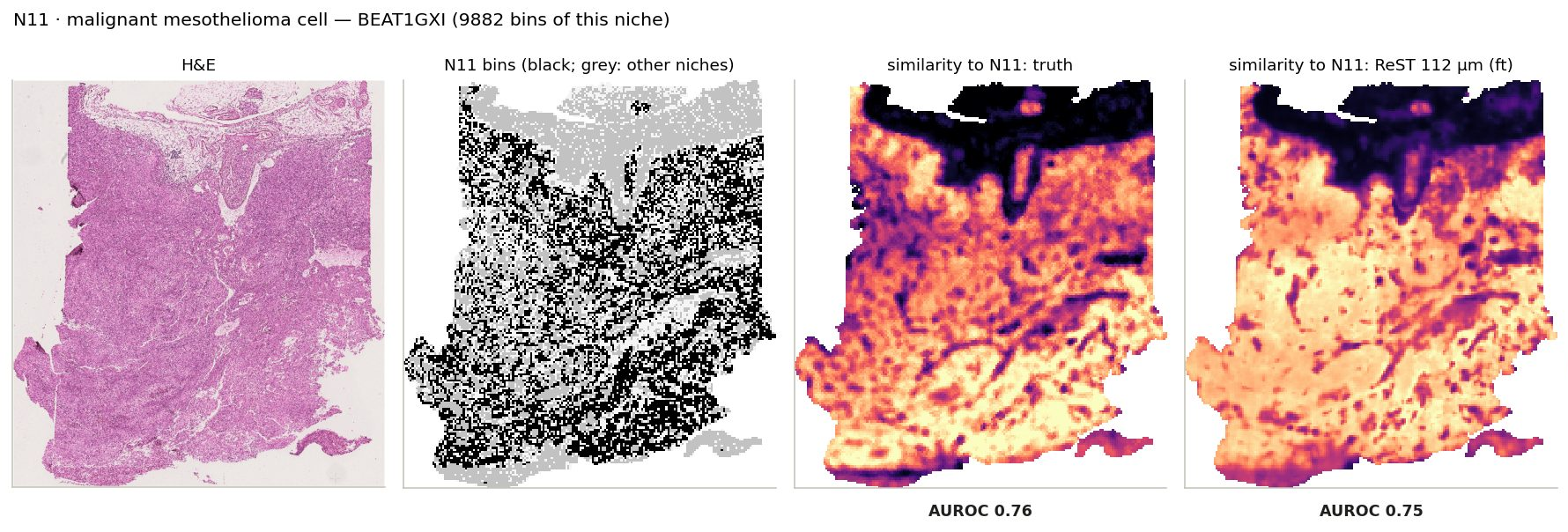
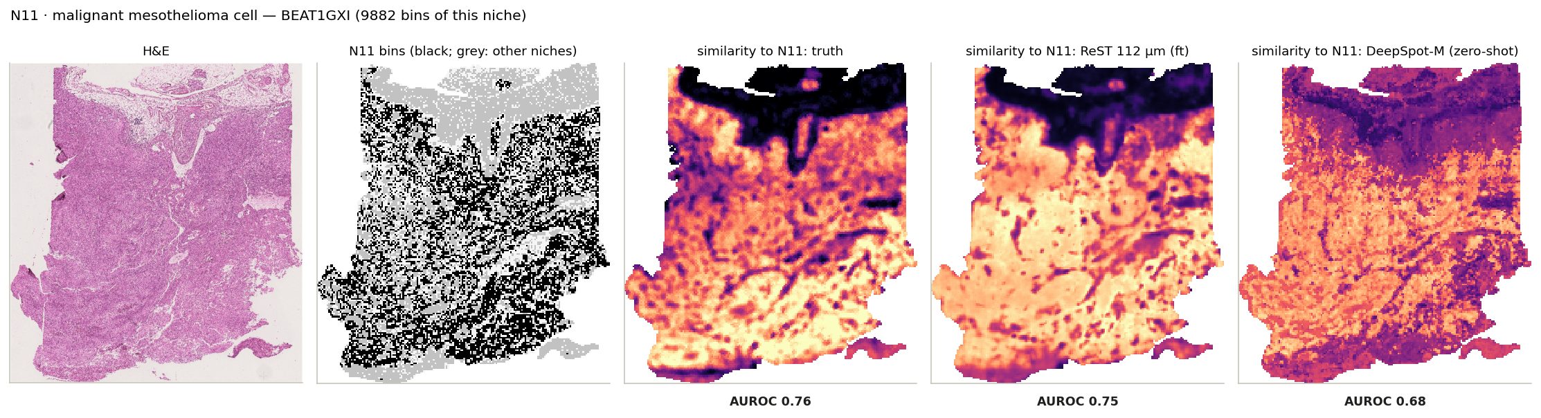
N11 · malignant mesothelioma cell: its bins on the slide where it is largest, and every bin's similarity to its centroid from the truth and from ReST.
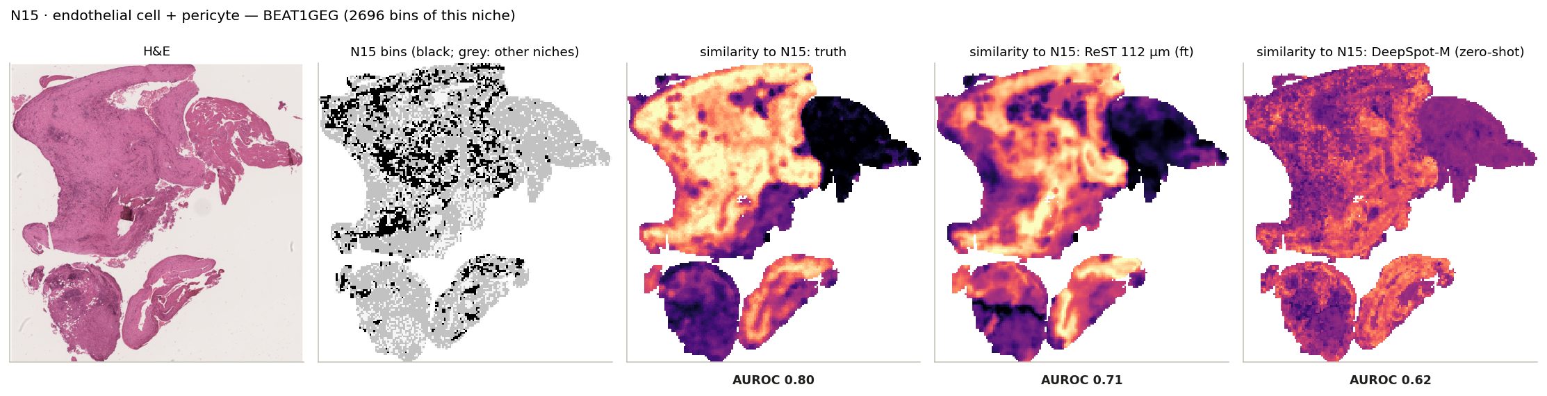
N15 · endothelial cell + pericyte: its bins on the slide where it is largest, and every bin's similarity to its centroid from the truth and from ReST.
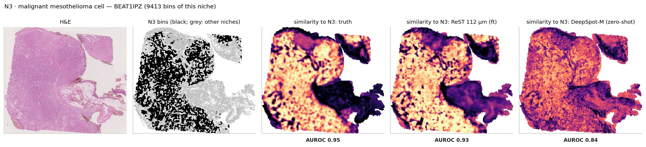
N3 · malignant mesothelioma cell: its bins on the slide where it is largest, and every bin's similarity to its centroid from the truth and from ReST.
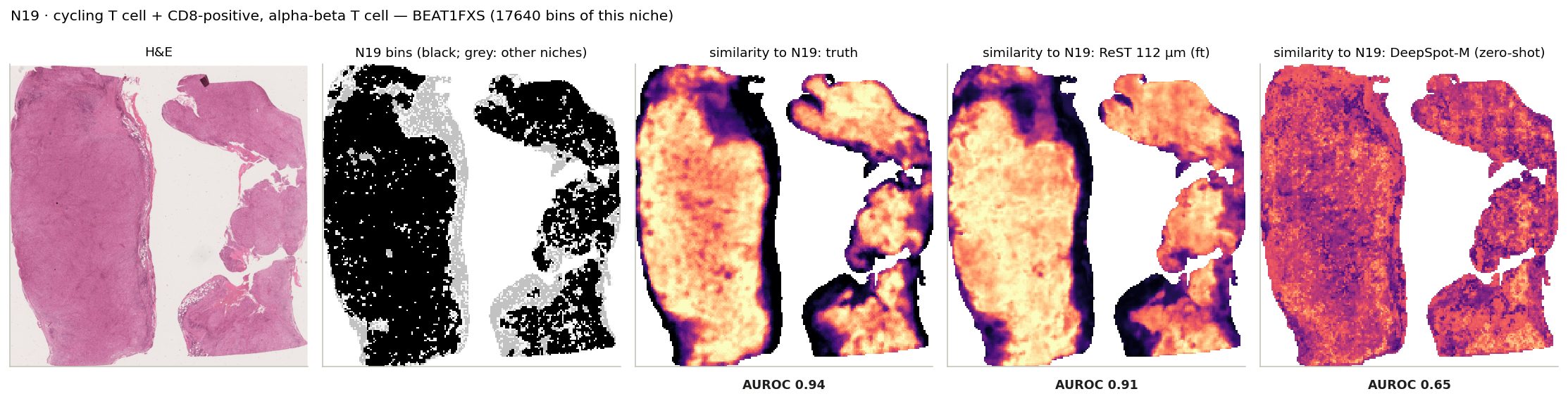
N19 · cycling T cell + CD8-positive, alpha-beta T cell: its bins on the slide where it is largest, and every bin's similarity to its centroid from the truth and from ReST.
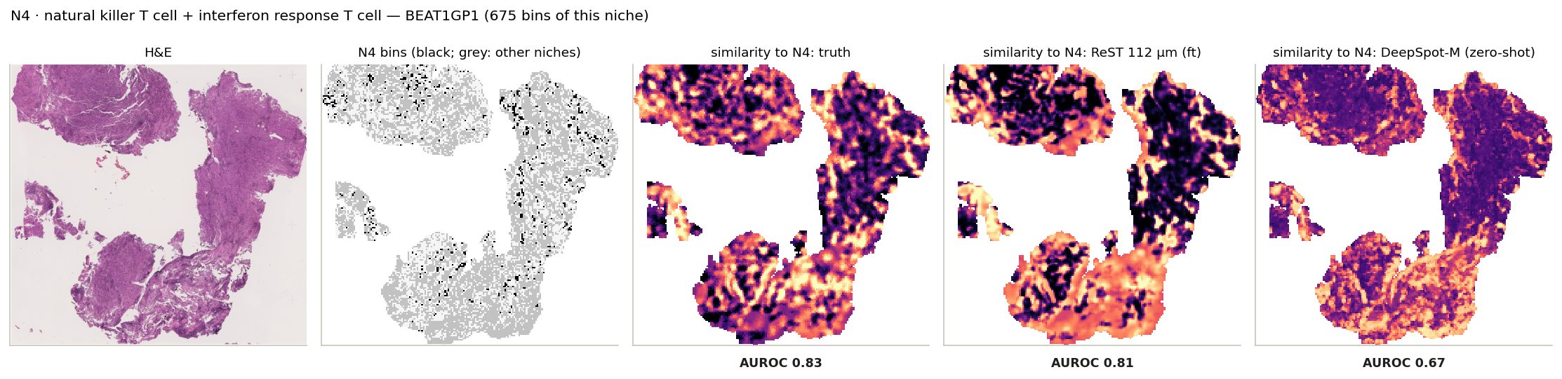
N4 · natural killer T cell + interferon response T cell: its bins on the slide where it is largest, and every bin's similarity to its centroid from the truth and from ReST.
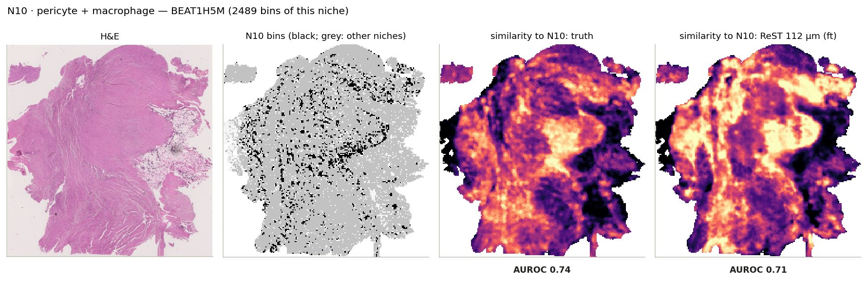
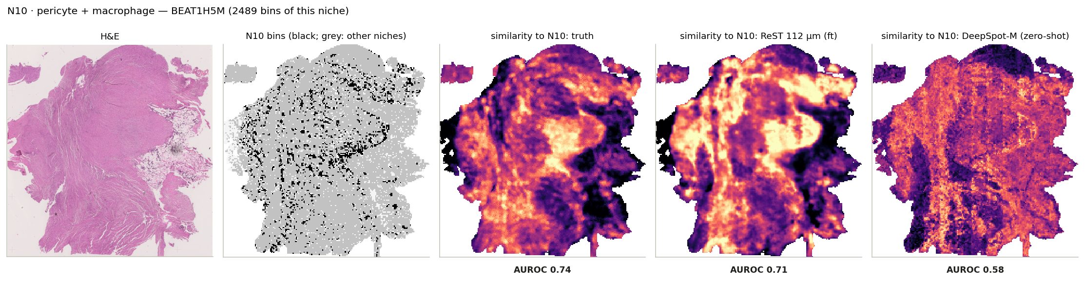
N10 · pericyte + macrophage: its bins on the slide where it is largest, and every bin's similarity to its centroid from the truth and from ReST.
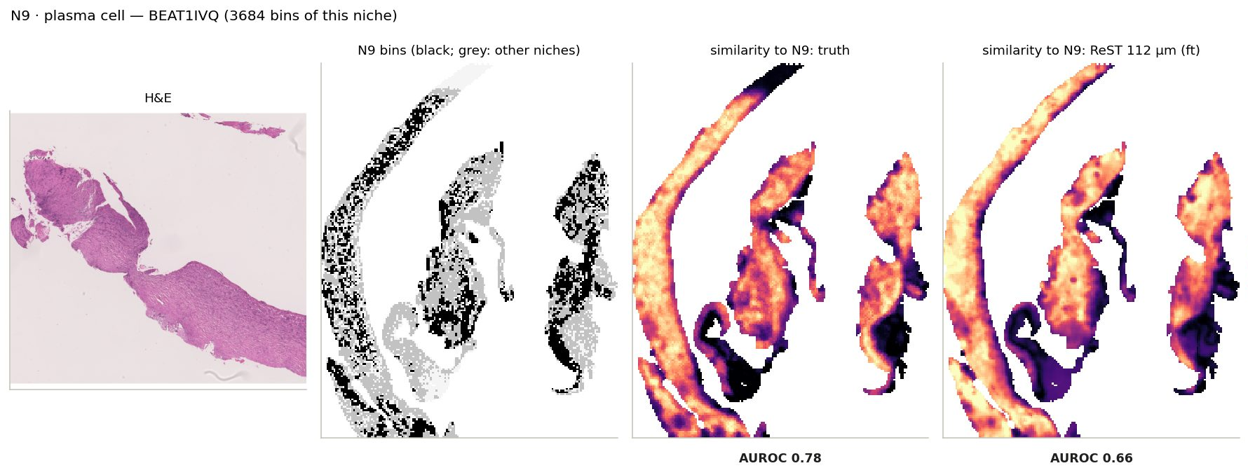
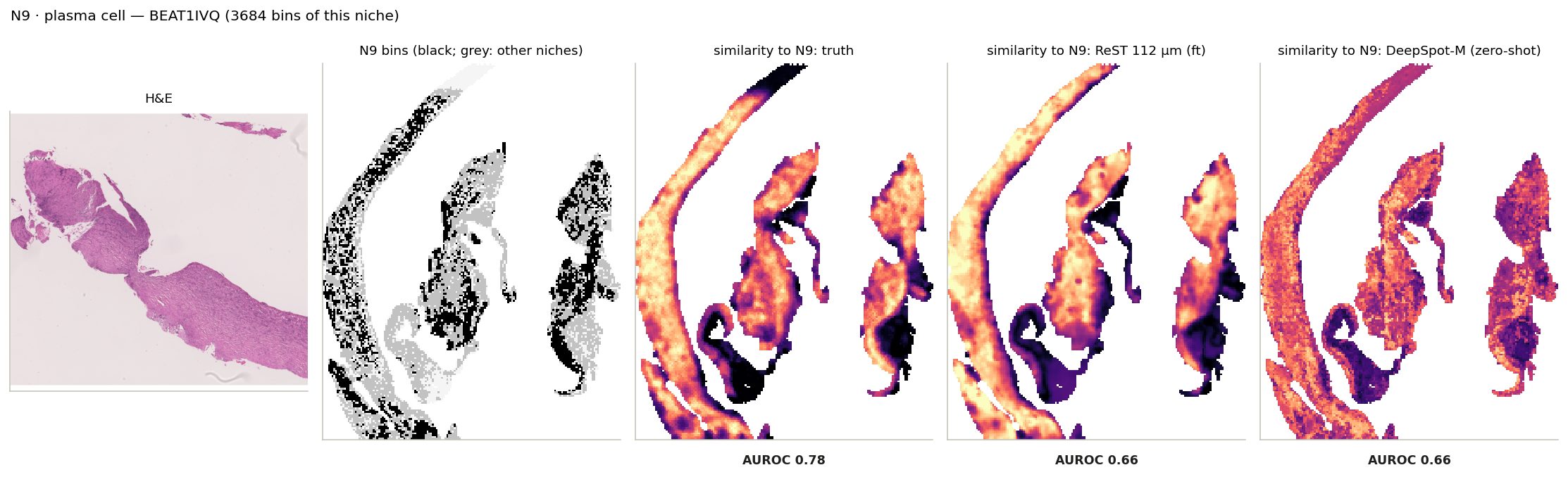
N9 · plasma cell: its bins on the slide where it is largest, and every bin's similarity to its centroid from the truth and from ReST.
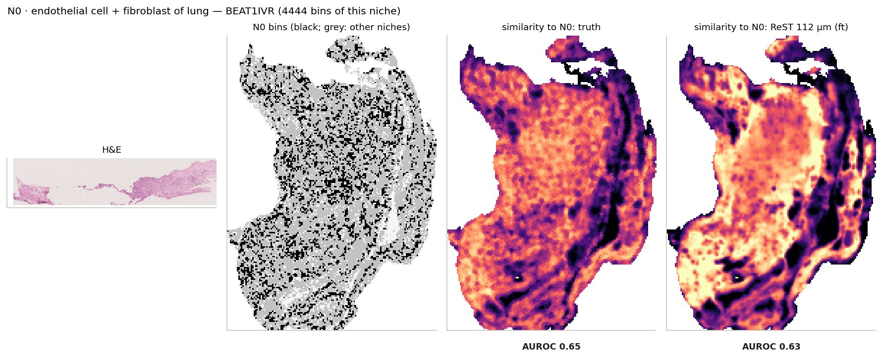
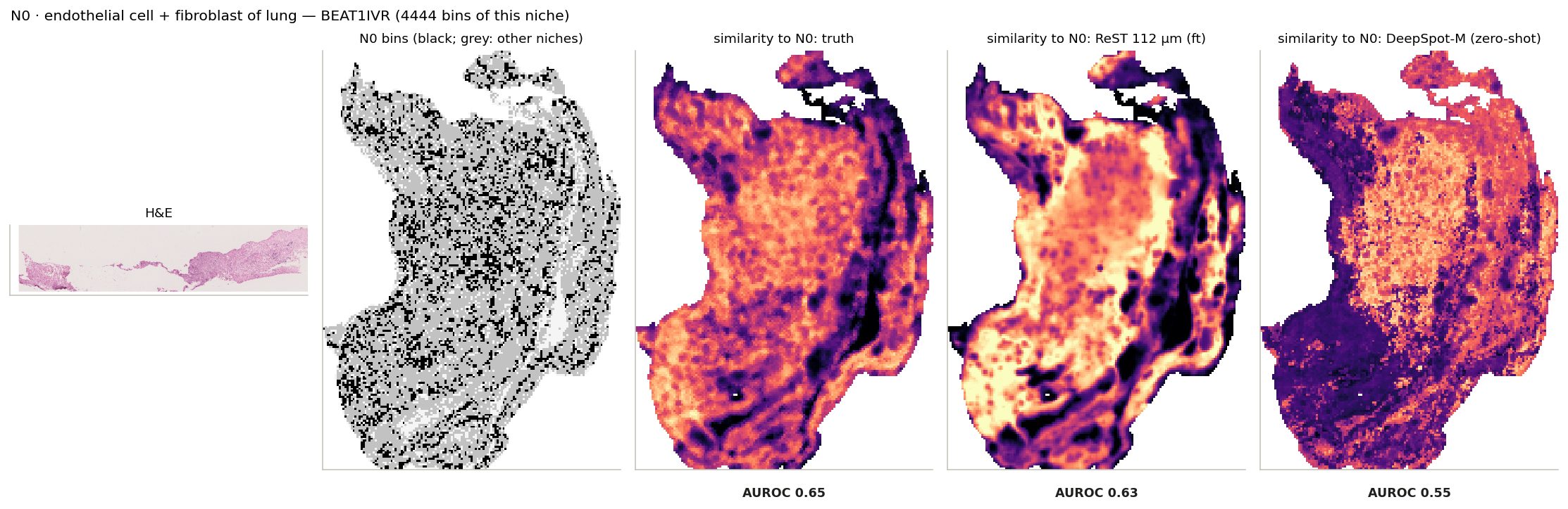
N0 · endothelial cell + fibroblast of lung: its bins on the slide where it is largest, and every bin's similarity to its centroid from the truth and from ReST.
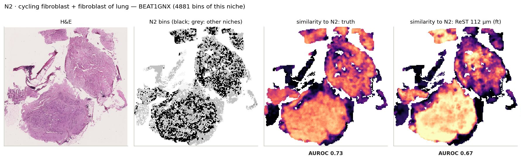
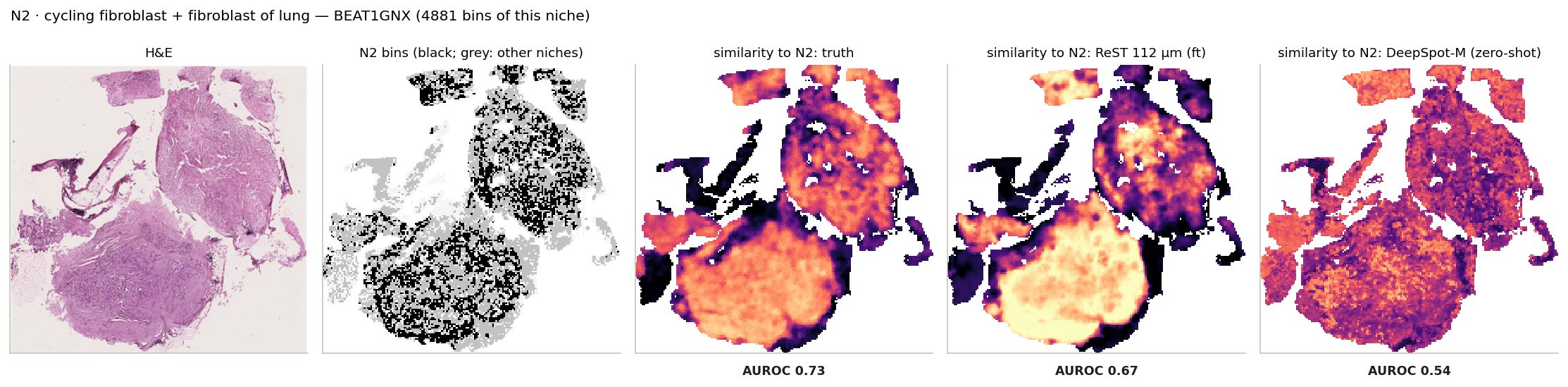
N2 · cycling fibroblast + fibroblast of lung: its bins on the slide where it is largest, and every bin's similarity to its centroid from the truth and from ReST.
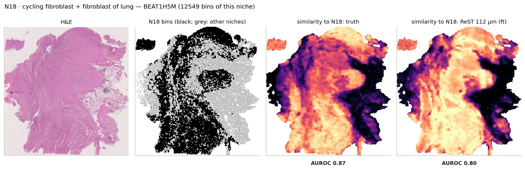
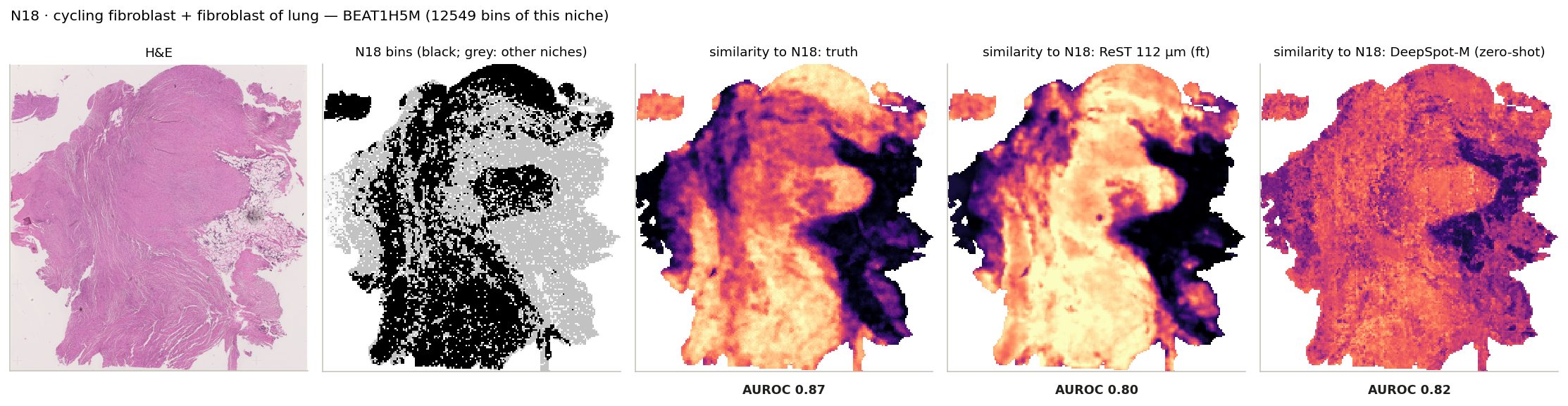
N18 · cycling fibroblast + fibroblast of lung: its bins on the slide where it is largest, and every bin's similarity to its centroid from the truth and from ReST.
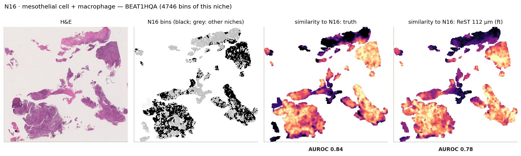
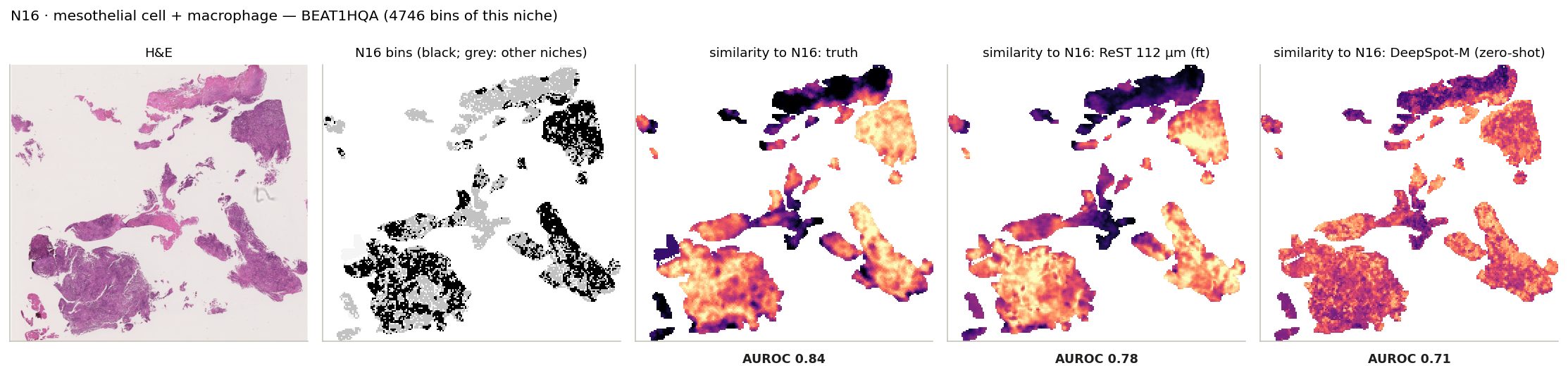
N16 · mesothelial cell + macrophage: its bins on the slide where it is largest, and every bin's similarity to its centroid from the truth and from ReST.
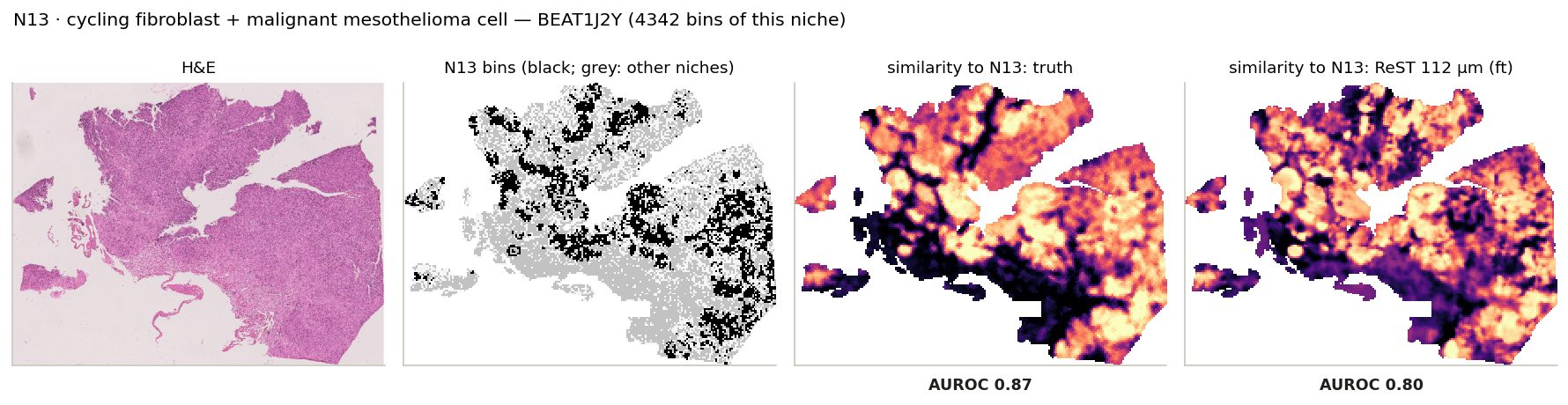
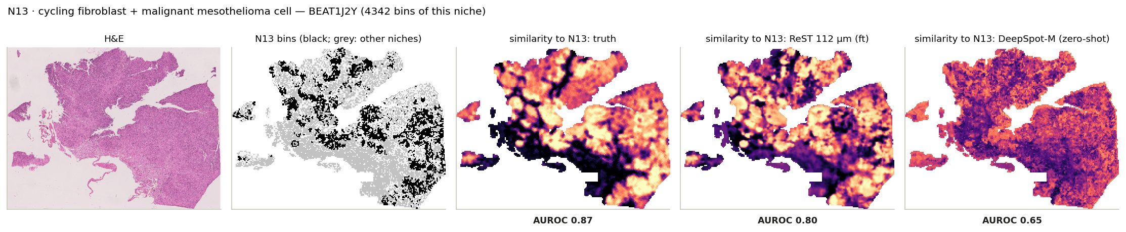
N13 · cycling fibroblast + malignant mesothelioma cell: its bins on the slide where it is largest, and every bin's similarity to its centroid from the truth and from ReST.
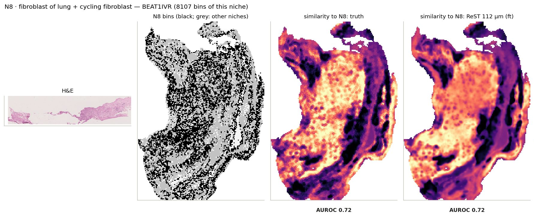
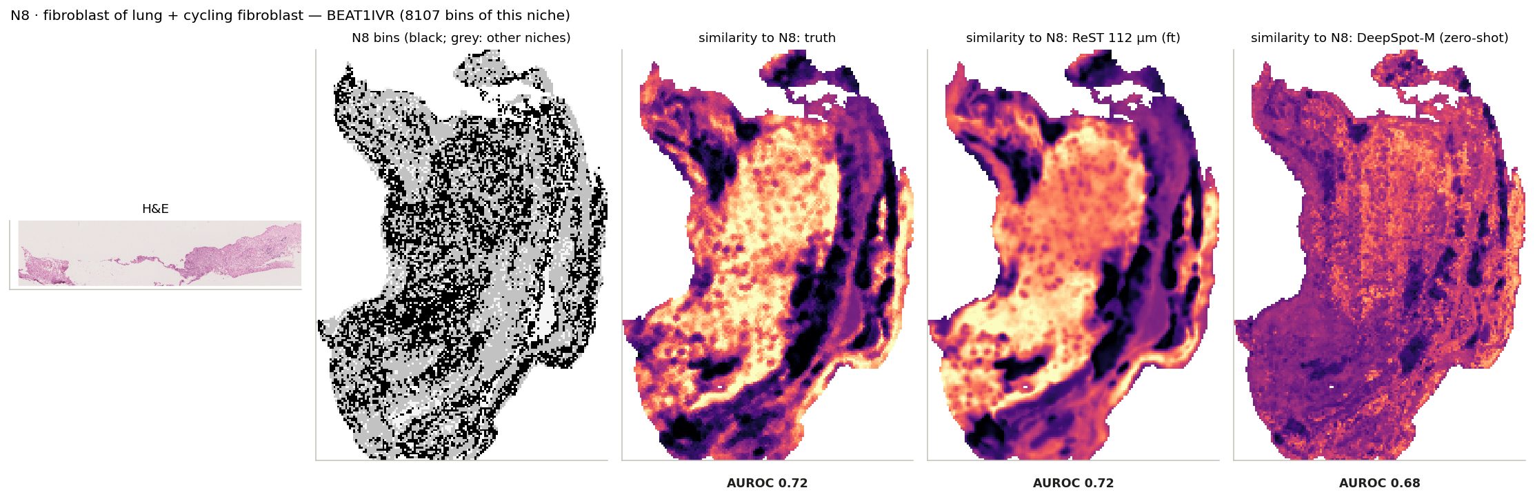
N8 · fibroblast of lung + cycling fibroblast: its bins on the slide where it is largest, and every bin's similarity to its centroid from the truth and from ReST.
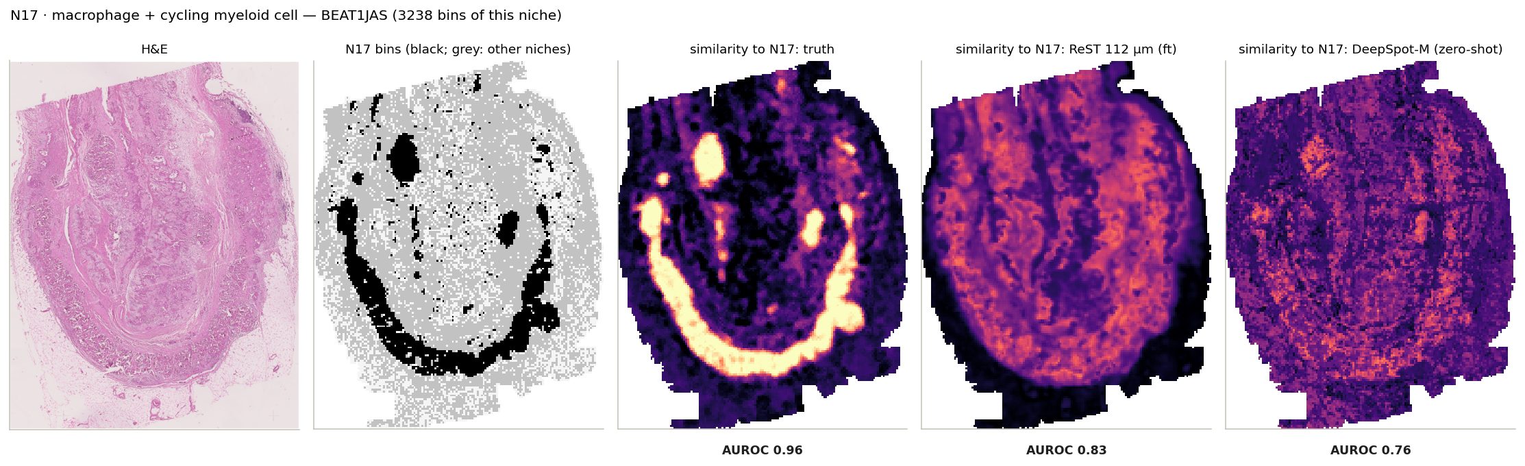
N17 · macrophage + cycling myeloid cell: its bins on the slide where it is largest, and every bin's similarity to its centroid from the truth and from ReST.
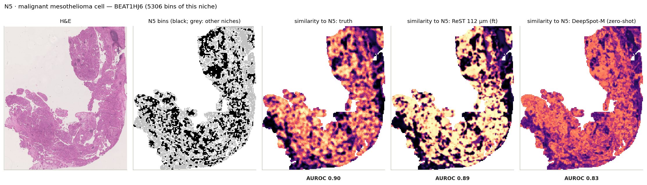
N5 · malignant mesothelioma cell: its bins on the slide where it is largest, and every bin's similarity to its centroid from the truth and from ReST.
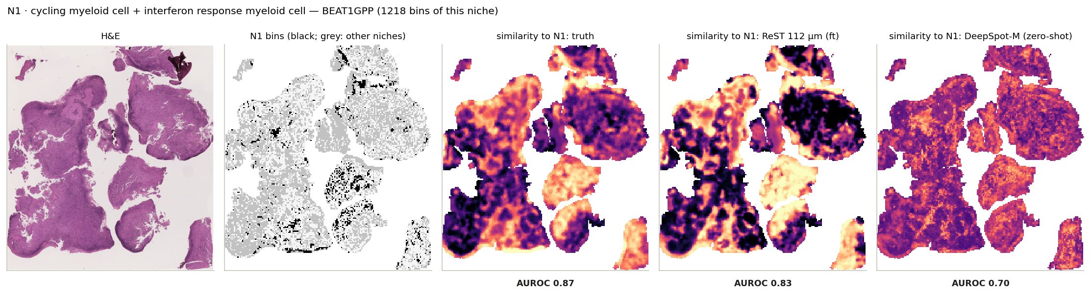
N1 · cycling myeloid cell + interferon response myeloid cell: its bins on the slide where it is largest, and every bin's similarity to its centroid from the truth and from ReST.
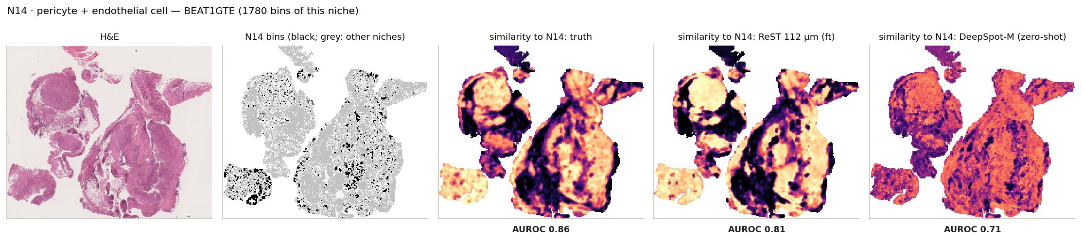
N14 · pericyte + endothelial cell: its bins on the slide where it is largest, and every bin's similarity to its centroid from the truth and from ReST.
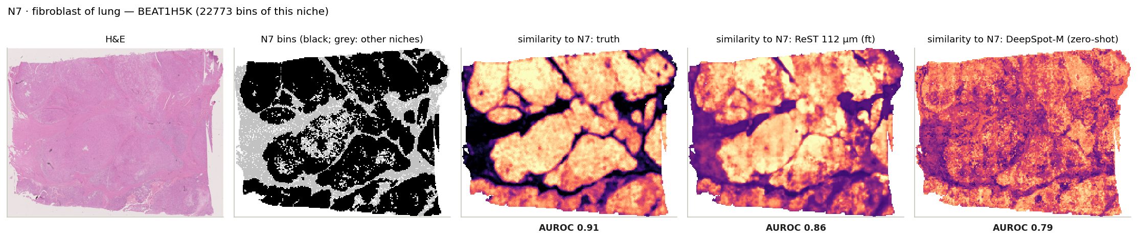
N7 · fibroblast of lung: its bins on the slide where it is largest, and every bin's similarity to its centroid from the truth and from ReST.
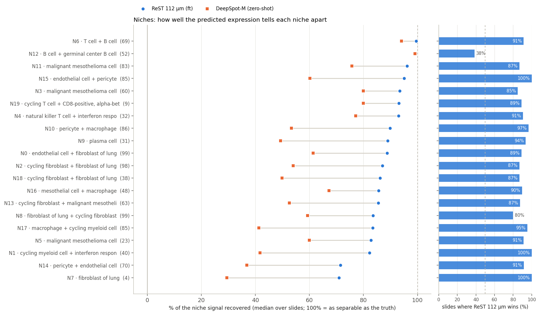
Niches: ReST recovers 88% of the signal
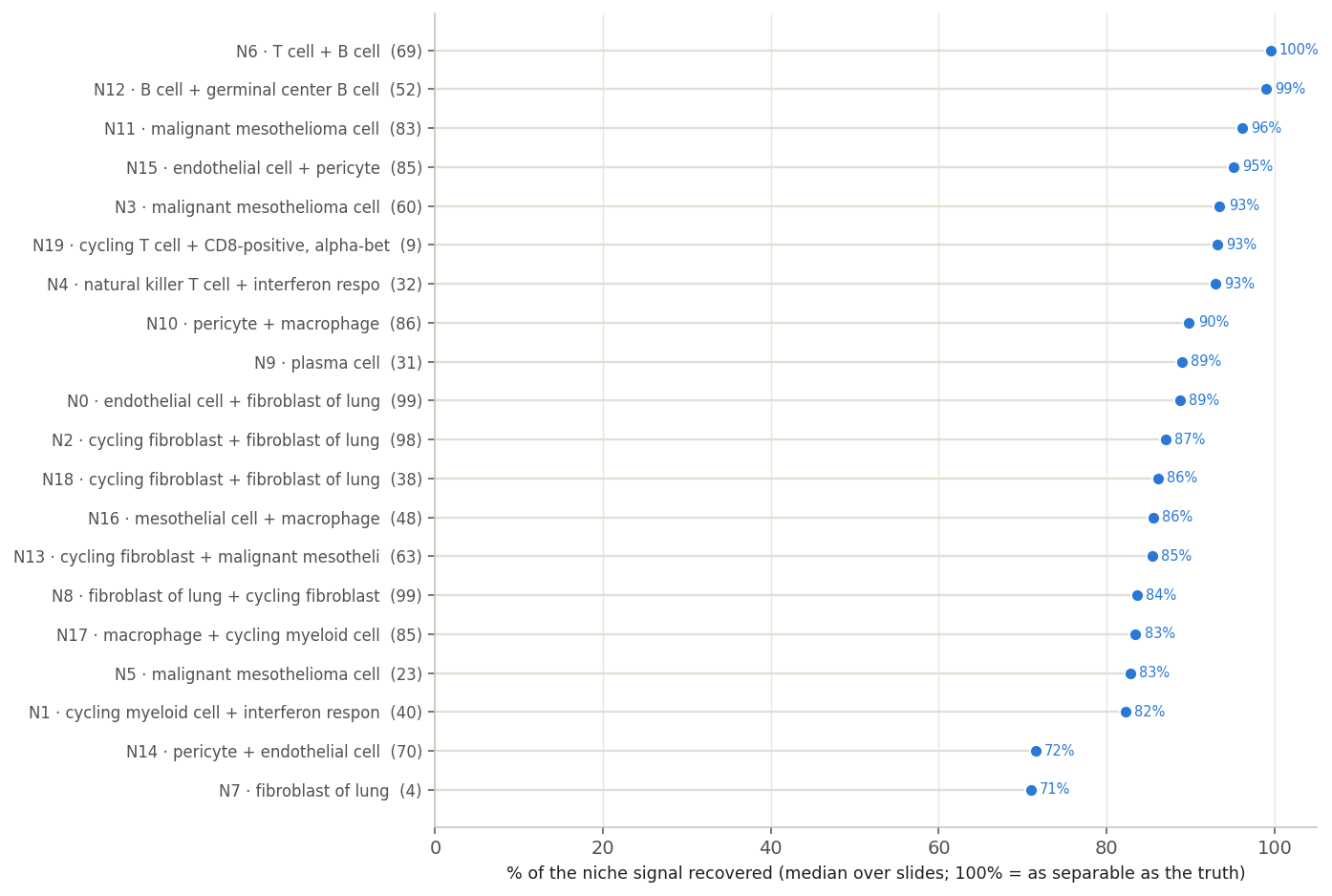
Median over slides, per niche.
88%
median niche
Easiest: N6 T cell + B cell, N12 B cell + germinal center B cell, N11 malignant mesothelioma cell. Hardest: N14 pericyte + endothelial cell, N7 fibroblast of lung.
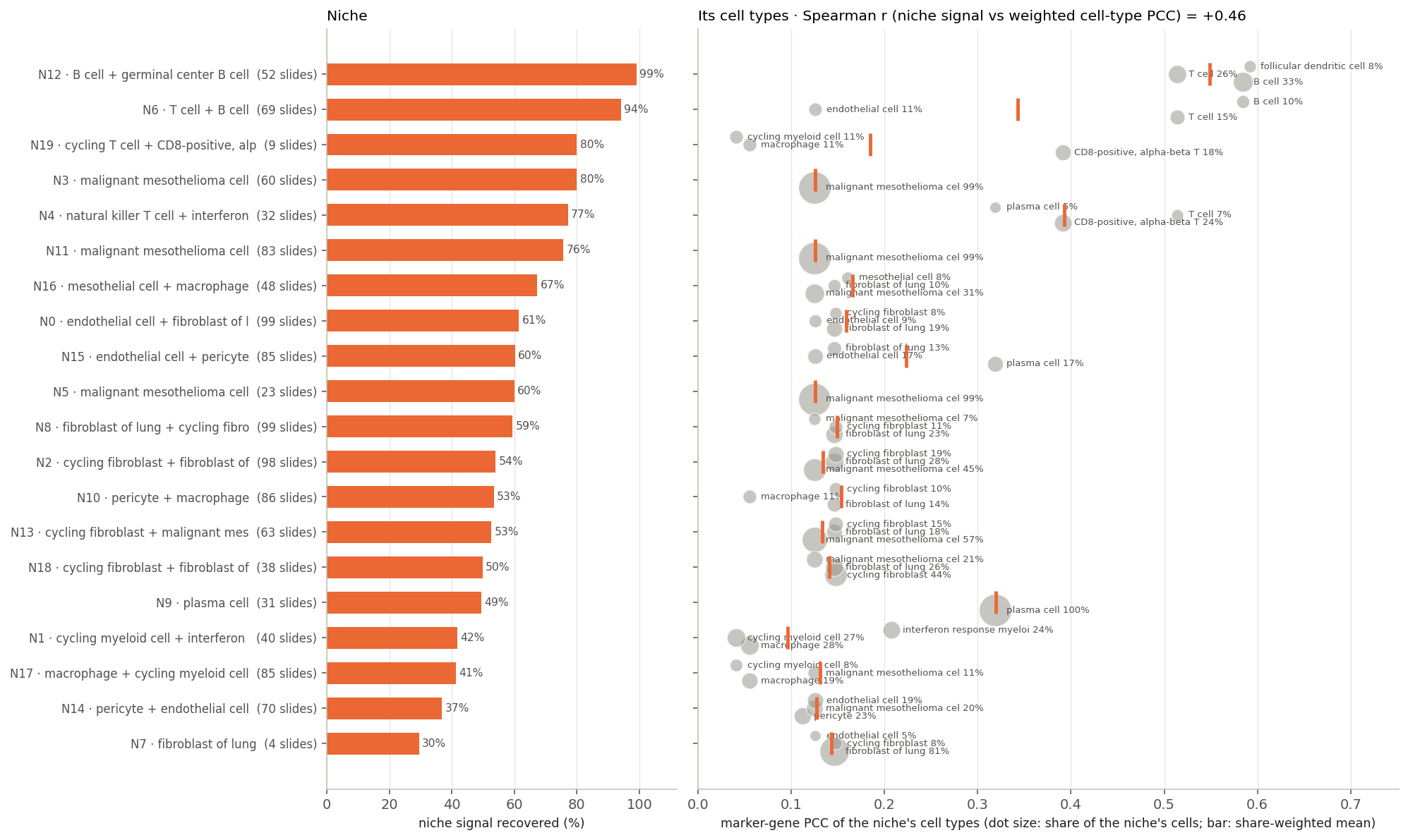
Niches and their cell types
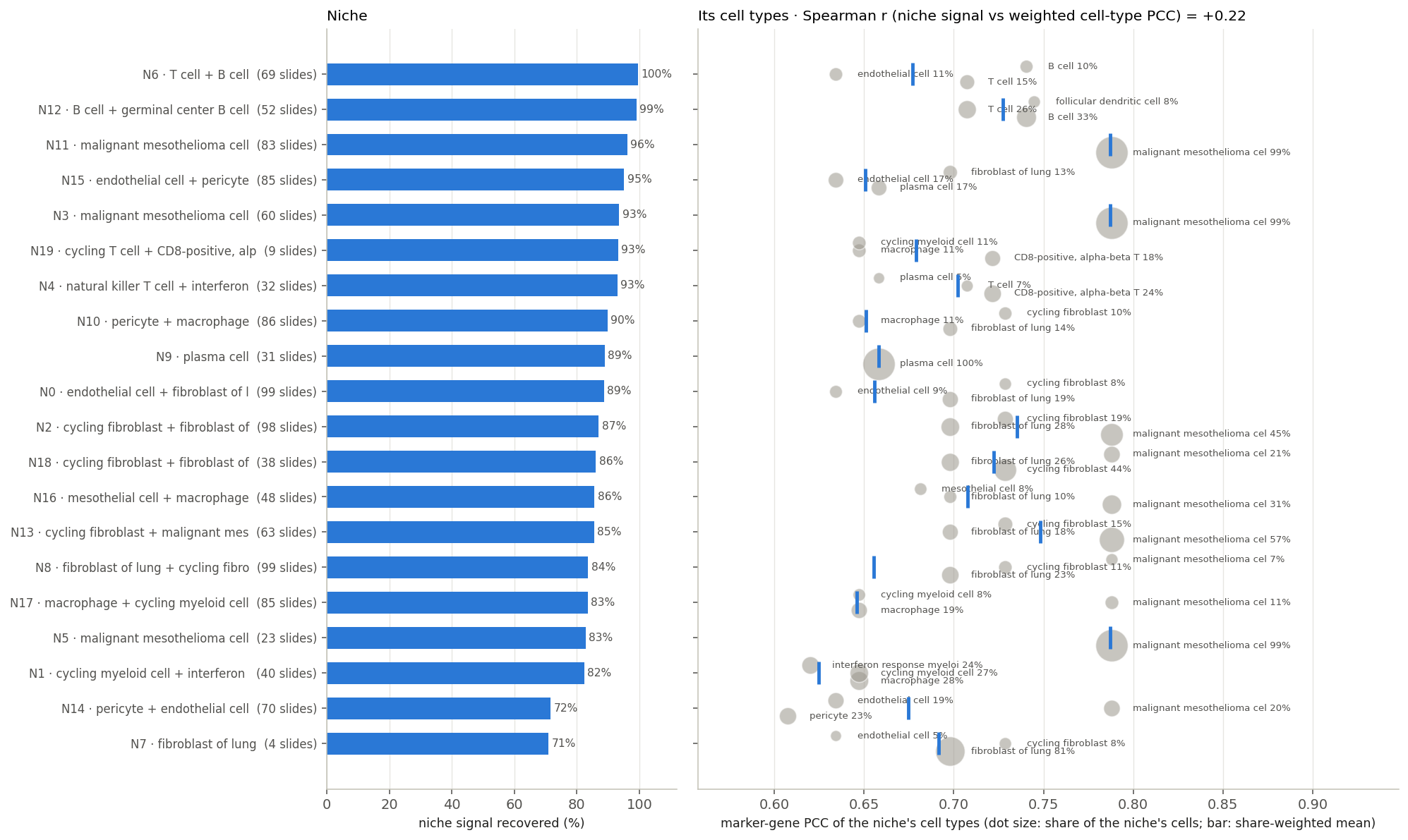
108 BEAT test slides. Marker PCC: median over all 108. Niche signal: median over the slides where the niche occurs (niche labels on 103)
Left: niche signal recovered (in brackets: slides where the niche occurs). Right: marker-gene PCC of each niche's main cell types (≥ 3% of its cells); dot size = share, bar = share-weighted mean.
One dot per niche: the two columns of the left figure against each other.
Spearman r
Rank the 20 niches twice: by signal recovered and by how well their cell types are predicted. r compares the two orders: +1 same order, 0 unrelated, −1 reversed.
ReST: r = +0.22. Its cell types are predicted at 0.62–0.79 in every niche, and that does not predict which niches are harder.
DeepSpot-M: r = +0.46, its niche recovery follows its cell-type accuracy.
Niches beyond H&E
Team’s groups by H&E visibility: 1 structure · 2 single cell · 3 cell mix · 4 the rest (108 BEAT slides)
Left: niche signal recovered. Right: niche profile, prediction vs truth (PCC across genes).
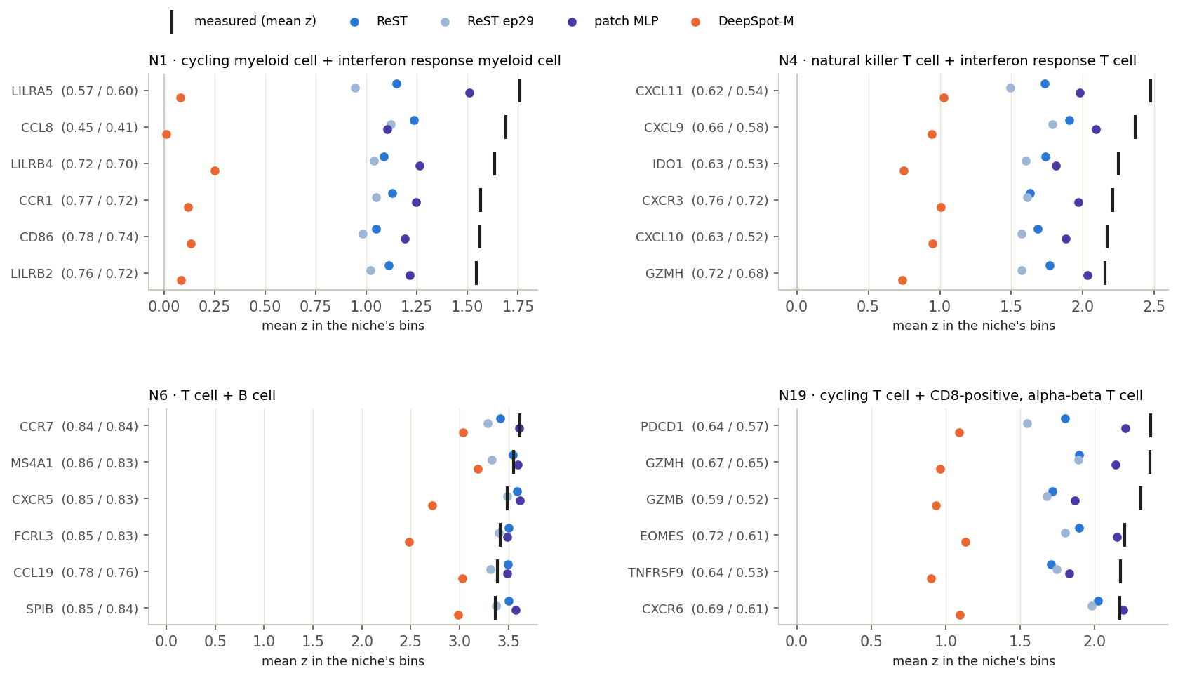
Mean z in the niche’s bins: measured (black) vs each model. Brackets: marker-map PCC, ReST / MLP.
group 4
N1 IFN-response myeloidN4 NKT + IFN-response TN6 T + B aggregatesN19 cycling CD8 T
93% · 94%
niche separated, ReST · MLP
23 / 24
marker maps where ReST beats the MLP
78% · 89%
marker contrast reached, ReST · MLP
Right genes in the right places; weaker peak than the MLP.
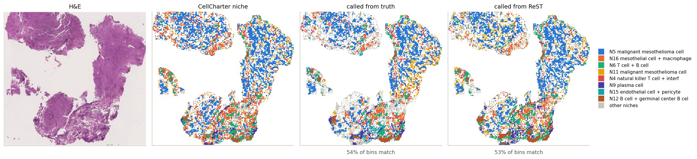
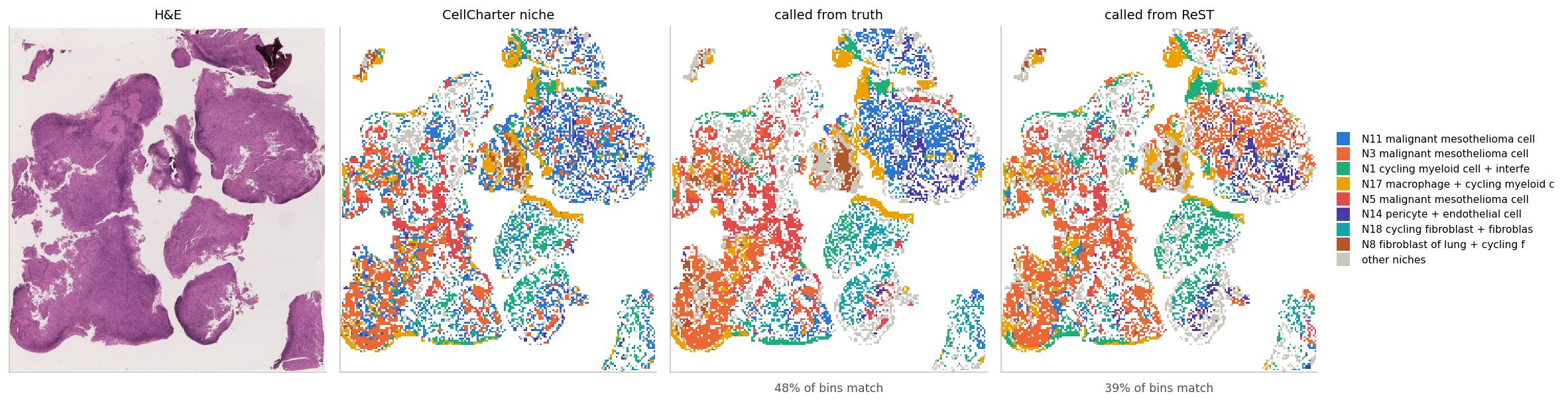
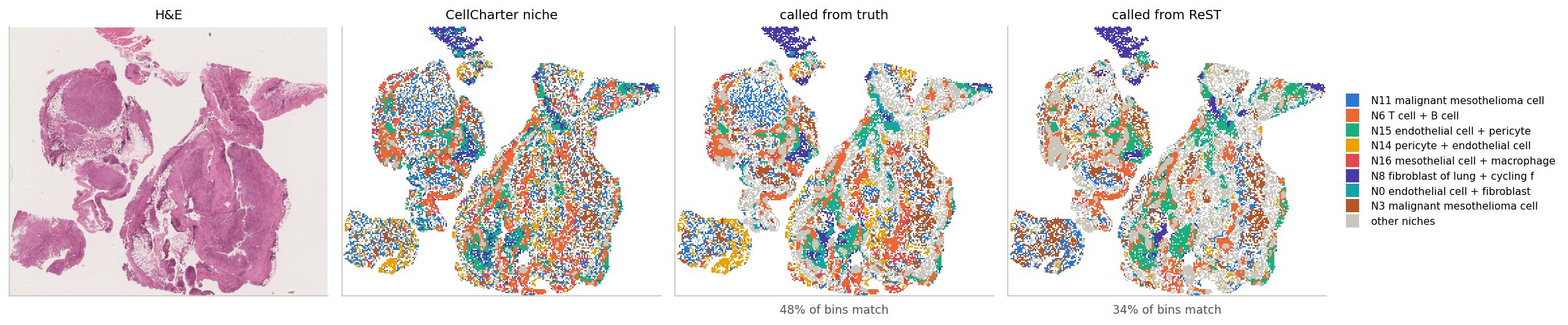
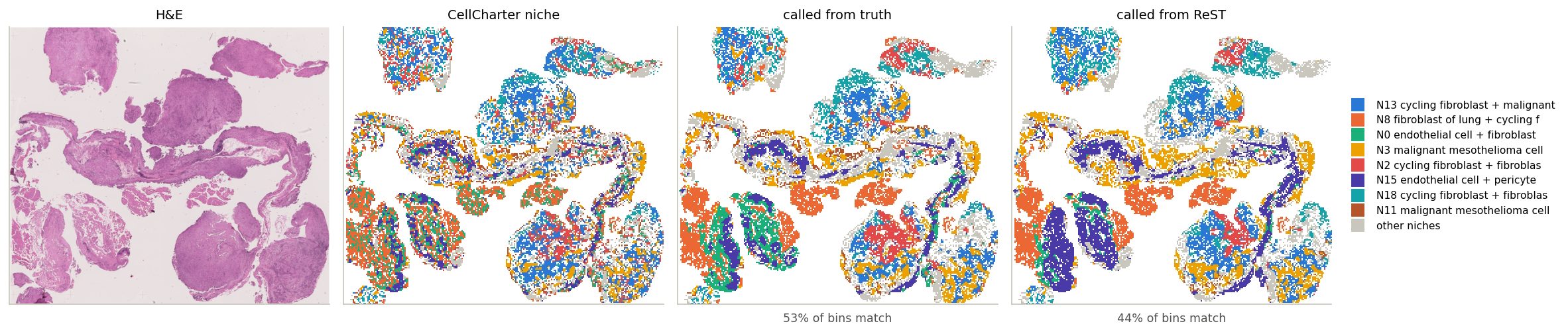
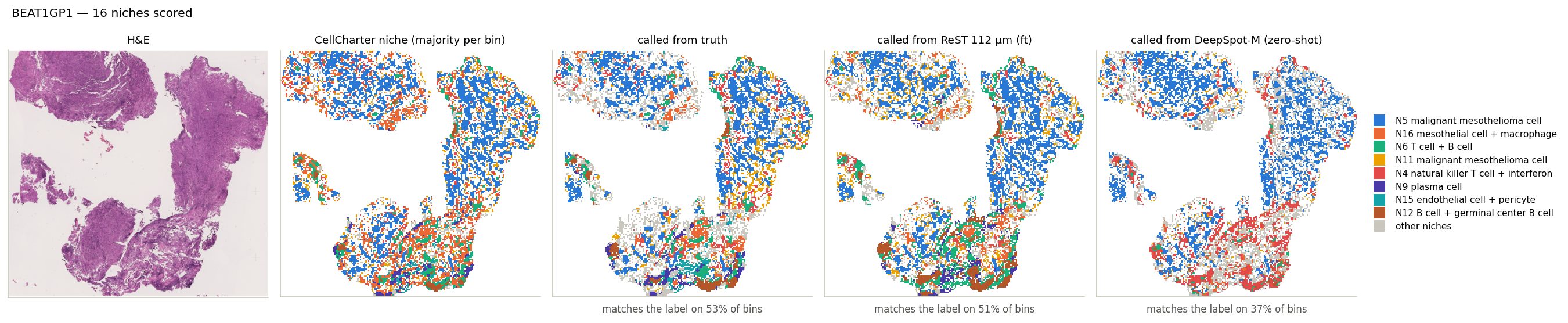
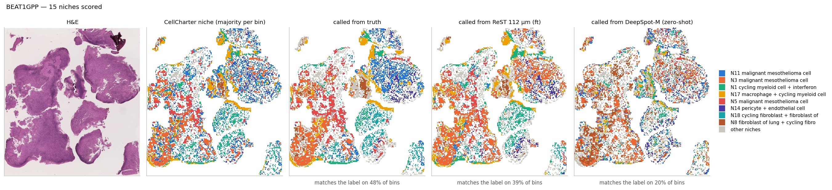
Niche calls, slide by slide
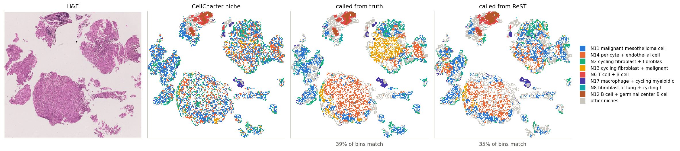
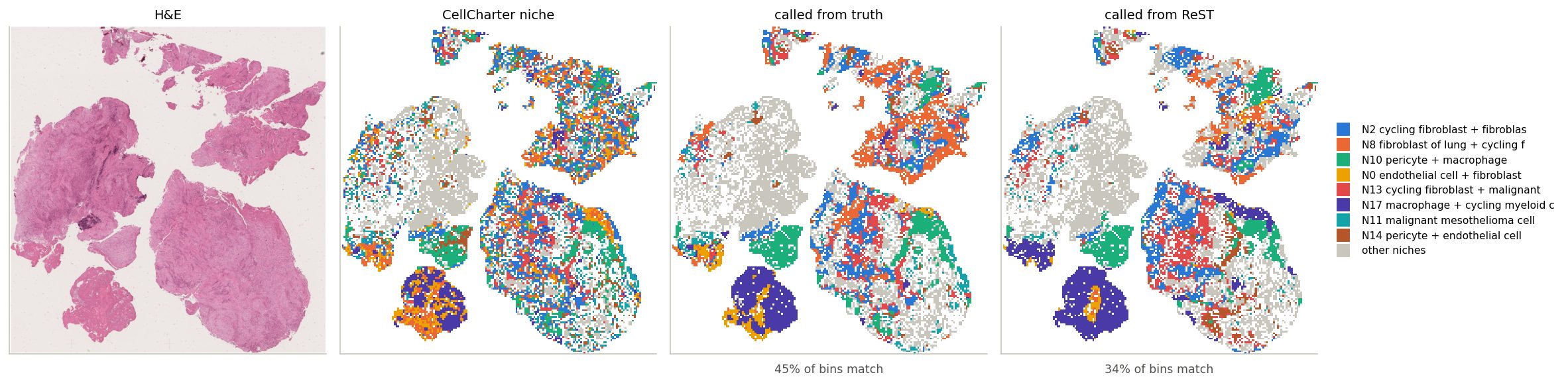
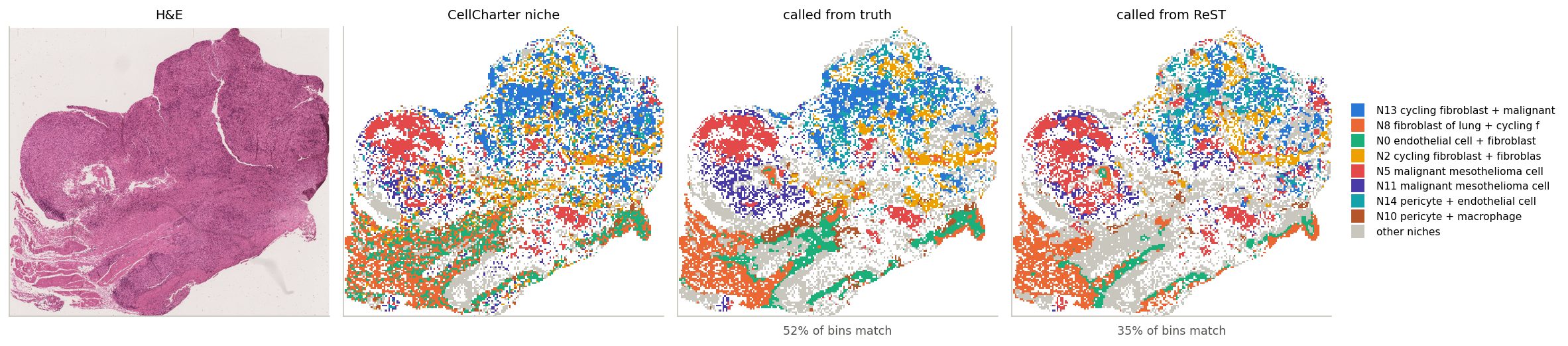
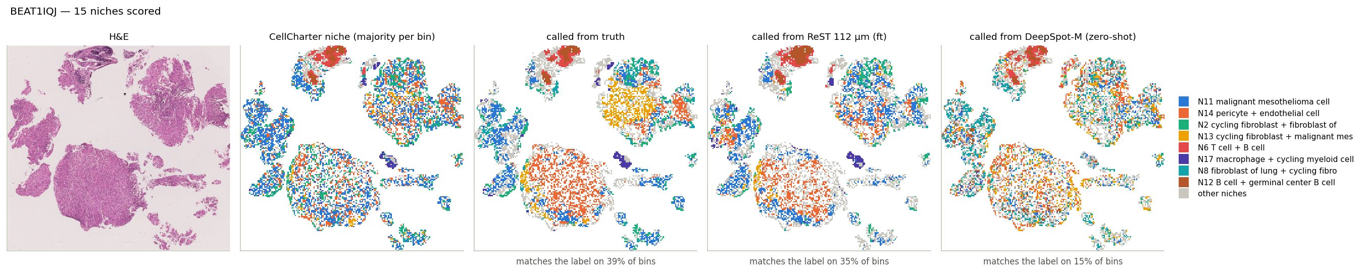
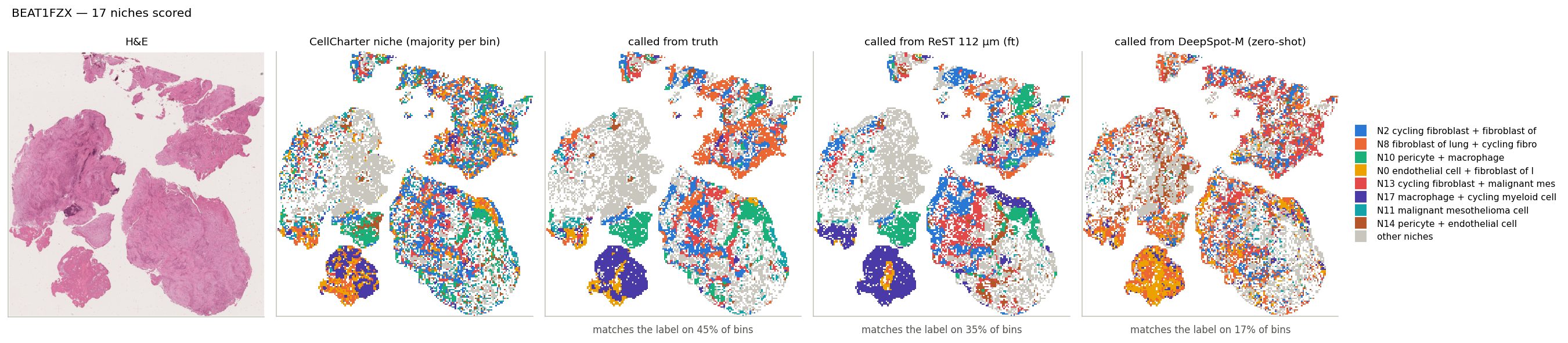
Each bin labelled by the niche centroid it resembles most; click a slide ID
CellCharter niche
The reference. A bin takes the niche of ≥ 50% of its cells (CellCharter labels cells from their own and their neighbours' expression). Mixed bins: blank.
called from truth
Each bin's measured expression, assigned to the most similar niche centroid (PCC across genes). The reference, not a ceiling: ReST predicts all bins jointly, so its bins carry context and beat it on 11% of niche-slide pairs.
called from ReST
The same rule on ReST's predicted expression (z-scored per gene over the slide), with the same centroids from the measured data. Compare with the middle map, “called from truth”.
Percentages: bins whose call matches the CellCharter niche. Colours: the slide's 8 most common niches; grey: the rest.
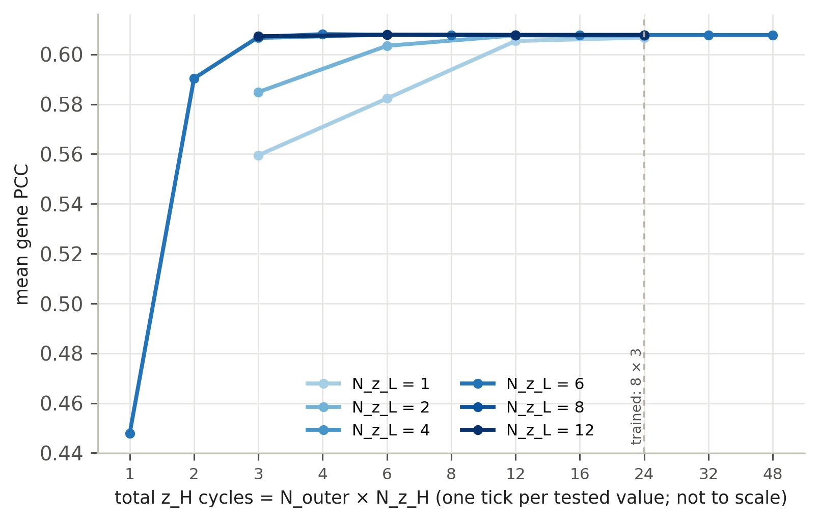
N_outer and N_z_H act the same: only their product, the total number of z_H cycles, matters.
Accuracy saturates at ~4 cycles: 15 calls give 0.607 mean gene PCC vs 0.608 at the trained 168.
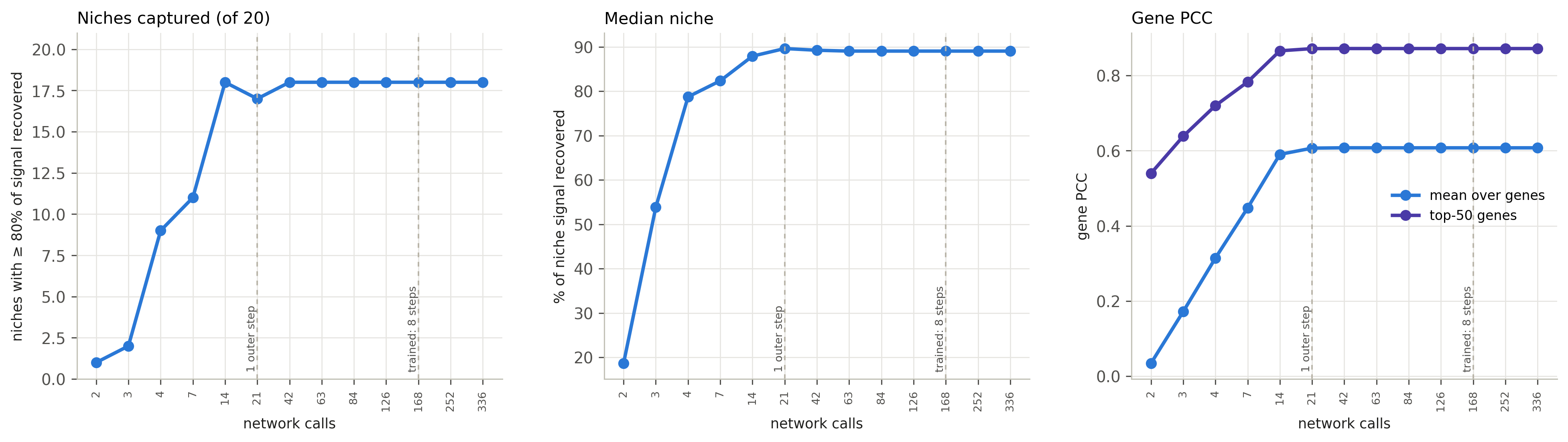
One checkpoint (ReST ep29, trained with 168 calls), 40 settings; same 108 BEAT patients. The deck's ReST runs at depth 4 (84 calls).
More recursion, more niches captured — up to one outer step
2 calls: 1 niches captured, gene PCC 0.03; 21 calls: 17, 0.61; beyond 42 calls nothing changes. x-axis: one tick per tested depth, not to scale.
19%
median niche recovered at 2 calls
82%
at 7 calls (one z_H cycle)
90%
at 21 calls (one outer step)
89%
at 168 calls (trained)
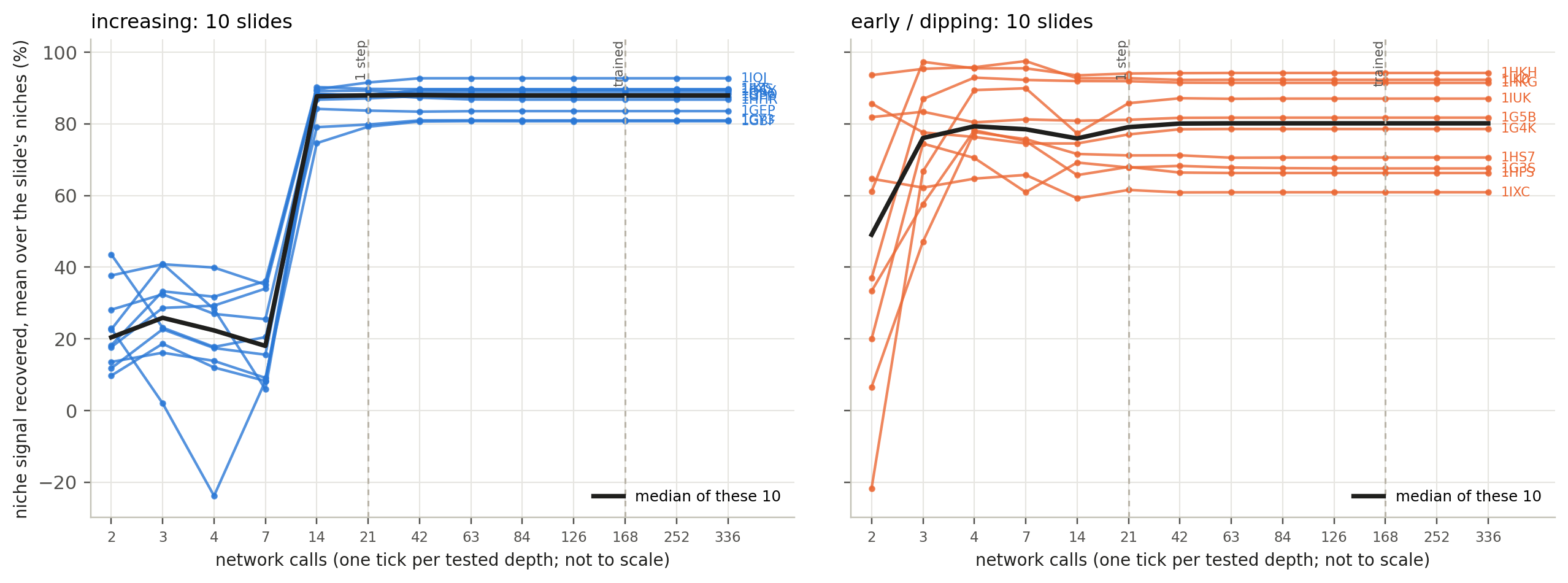
Where depth matters, and where it does not
Left: 10 slides with the largest gain from 7 to 168 calls (+54 to +81 points). Right: 10 slides within 2 points of their best by 4 calls, then dropping up to 12.
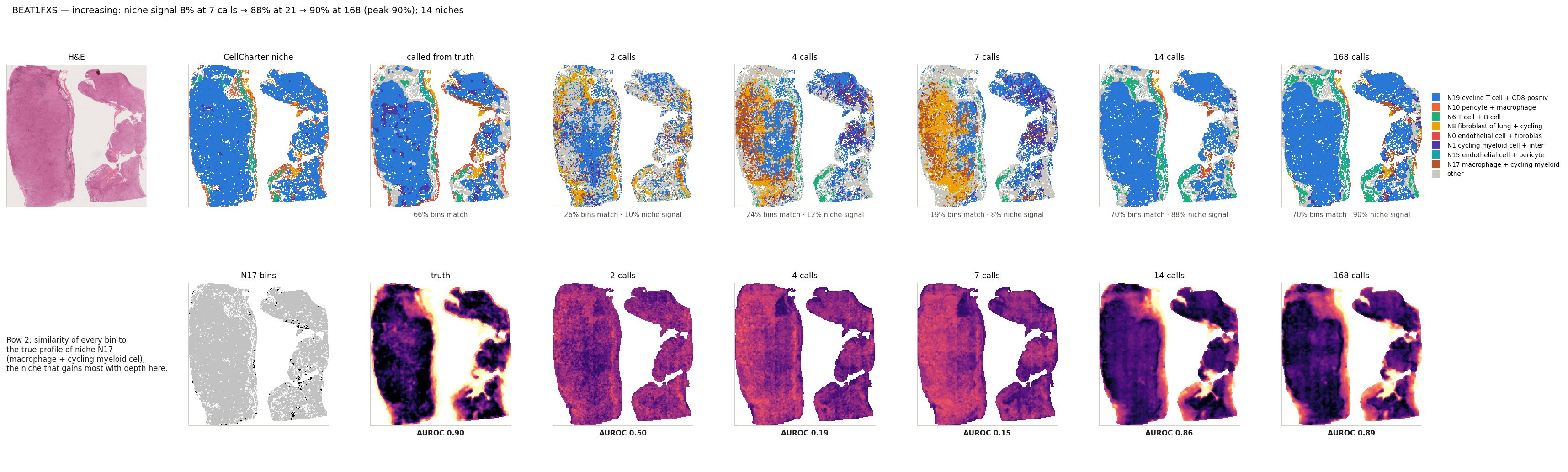
Depth helps: BEAT1FXS
Niche signal 8% at 7 calls → 88% at 21 → 90% at 168 · gene PCC -0.03 → 0.58 → 0.59
Top: niche calls at each depth. Bottom: similarity to the macrophage + cycling myeloid niche.
CellCharter niche: bin label from its cells · called from truth: nearest niche centroid from the measured expression (reference) · N calls: the same from ReST stopped after N network calls. Under each map: bins matching CellCharter, niche signal recovered.
BEAT1FXS
2 calls
4 calls
7 calls
14 calls
21 calls
168 calls
niche signal recovered
10%
12%
8%
88%
88%
90%
mean gene PCC
0.015
-0.043
-0.030
0.566
0.584
0.585
top-50 gene PCC
0.525
0.517
0.599
0.874
0.898
0.890
Bold: best depth on this slide. 21 calls = one outer step; 168 = trained (8 steps).
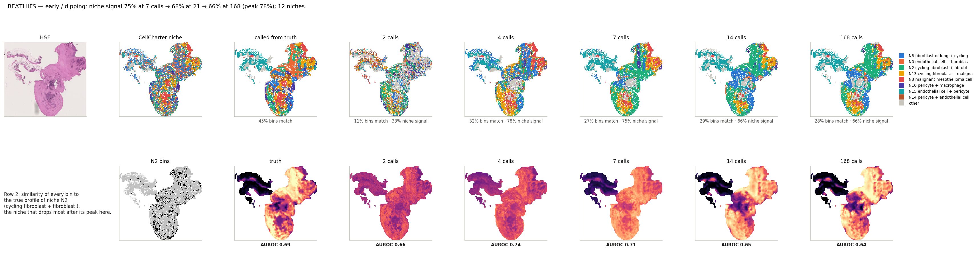
Saturates early: BEAT1HFS
Niche signal 78% at 4 calls → 68% at 21 → 66% at 168 · gene PCC 0.43 → 0.64 → 0.65 (keeps rising)
Top: niche calls at each depth. Bottom: similarity to the cycling fibroblast niche, the one that drops most.
CellCharter niche: bin label from its cells · called from truth: nearest niche centroid from the measured expression (reference) · N calls: the same from ReST stopped after N network calls. Under each map: bins matching CellCharter, niche signal recovered.
BEAT1HFS
2 calls
4 calls
7 calls
14 calls
21 calls
168 calls
niche signal recovered
33%
78%
75%
66%
68%
66%
mean gene PCC
-0.048
0.429
0.583
0.630
0.640
0.645
top-50 gene PCC
0.473
0.794
0.884
0.897
0.912
0.912
Bold: best depth on this slide. 21 calls = one outer step; 168 = trained (8 steps).
Summary
1BEAT, 108 held-out patients: median gene PCC 0.75; add-on genes predicted as well as the 10x panel.
2Cell-type markers: median PCC 0.65 over 23 cell types.
3Pathways: median PCC 0.64, active-region IoU 0.27 (chance 0.09). Niches: 88% of the signal recovered.
4Recursion matters up to ~4 z_H cycles; the trained 8 outer steps add nothing beyond that.
Reality check: BEAT and 10x test slides come from cohorts ReST trained on (other patients).
Extras
Additional analyses, not part of the main story.
Which genes does spatial context help?
Each dot is a gene (size: expression). x: against the smoothed truth used in training; y: against unsmoothed counts.
comparison
ReST vs the patch MLP on the same 112 µm patches and slides, and vs the MLP's prediction averaged over each bin's 10 nearest bins (smoothing, no learning). 108 BEAT patients, 448 expressed genes.
Reality check: most of ReST's edge over the MLP is what plain smoothing gives; the two models also differ in more than context.
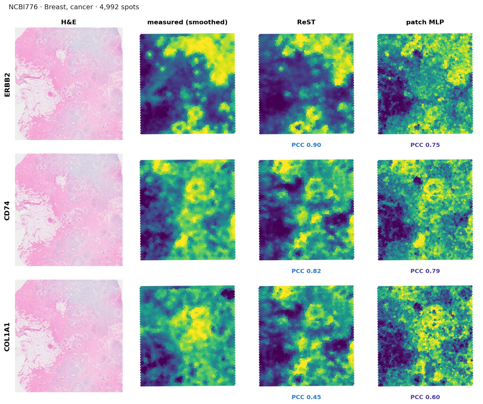
Transfer to Visium: one slide
setup
Data: 104 human Visium slides from HEST-1k, up to 3 per study, 16 organs
Never seen: no patient and no study ReST trained on
Input: 112 µm H&E crop around each 55 µm spot, as in training; spots are 100 µm apart
Truth: spot counts, log1p, averaged with the 6 neighbouring spots (training truth is smoothed too)
Models: ReST and the patch MLP, both trained on Xenium only; no fine-tuning
Metric: PCC per gene across a slide's spots — higher is better
Each map scaled to its own 2nd–98th percentile; PCC across the slide's spots.
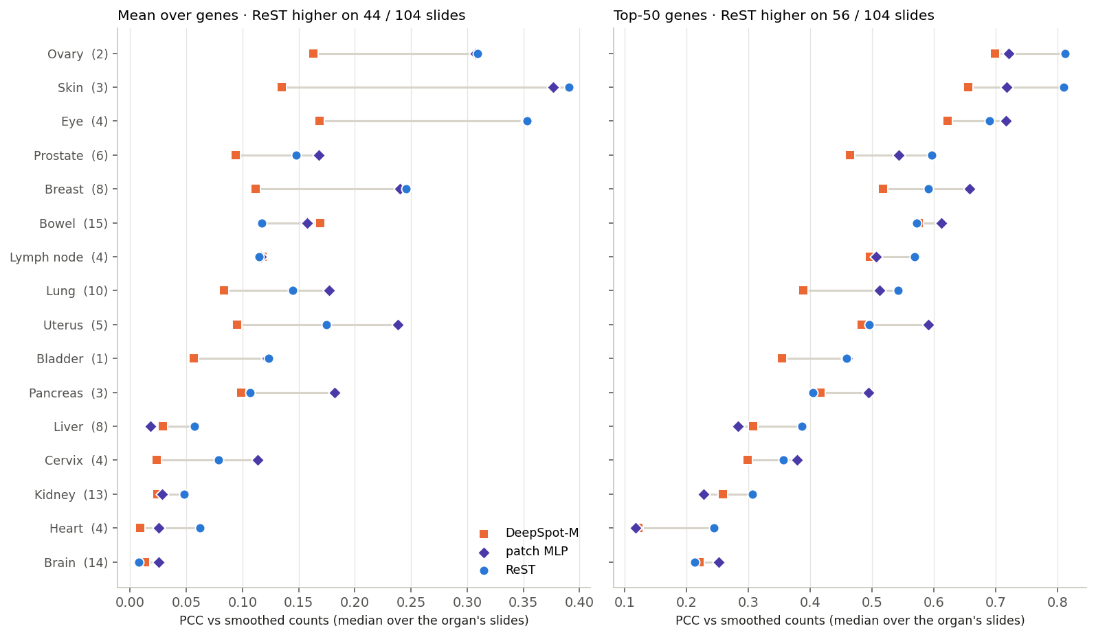
Transfer to Visium: by organ
ReST higher on its top-50 genes on 56 / 104 slides; the MLP higher on the mean over genes (44 / 104)
Organs sorted by ReST's top-50 PCC; in brackets: slides. All three models on the genes they all predict.
0.46 / 0.49
top-50 PCC, ReST / MLP (median slide)
0.11 / 0.14
mean PCC, ReST / MLP
ReST is higher on the top-50 genes on 56 / 104 slides, on the mean on 44.
Ovary, skin and eye transfer best; kidney, heart and brain worst (ReST top-50, organs with ≥ 2 slides). On BEAT Xenium the same ReST reaches 0.65 mean PCC.
DeepSpot-M
Trained on Visium (15 datasets, 14 cancers; HEST-1k not used); mean of its five gene-embedding sources: top-50 0.42, mean 0.08, below both Xenium-trained models. With evo2 only: top-50 0.40, mean 0.11.
Transfer to Visium: does the spot layout matter?
ReST ep29 (layout study): neither true spacing (B) nor filling the gaps (C) helps; the layout is not what limits ReST on Visium
Spot positions are rounded to the nearest 55 µm bin.
Median over 104 slides. A, B, C: ReST with the three layouts above; the MLP sees one patch and is unaffected by layout.
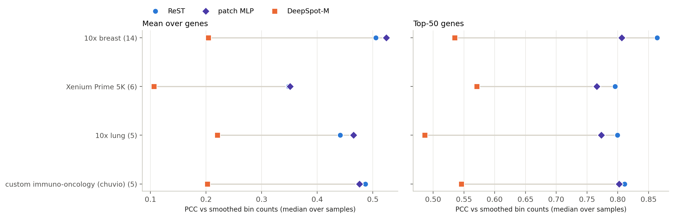
Transfer to SPLIT: breast and lung, never seen
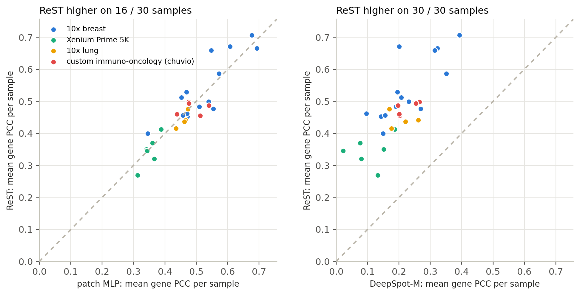
ReST higher than the MLP on its best genes (0.81 vs 0.80); level on the mean over genes (0.469 vs 0.471)
setup
Data: 30 Xenium samples from SPLIT (GSE311609) with registered H&E: 14 breast, 16 NSCLC
Panels: 10x breast, 10x lung, Xenium Prime 5K, a custom immuno-oncology panel
Never seen by any model; same 55 µm bins and 112 µm crops as every other set
Genes: the union-panel genes each panel measures (breast 280, lung 233, 5K 826, immuno-oncology 294)
Metric: PCC per gene across a sample's bins — higher is better
0.81 / 0.80 / 0.54
top-50 PCC: ReST / MLP / DeepSpot-M
0.47 / 0.47 / 0.20
mean PCC: ReST / MLP / DeepSpot-M
Median per sample. ReST higher than DeepSpot-M on 30 / 30 samples; than the MLP on 24 (top-50) and 16 (mean).
SPLIT: one sample per panel
Click a sample: H&E, measured, ReST, MLP and DeepSpot-M maps
Each dot is one sample; above the diagonal = ReST higher.
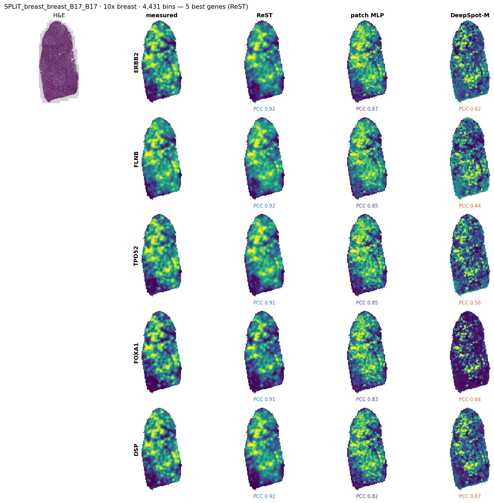
SPLIT_breast_breast_B17_B17 (10x breast, median sample of its panel by ReST top-50): its 5 best genes for ReST, with the MLP and DeepSpot-M on the same genes.
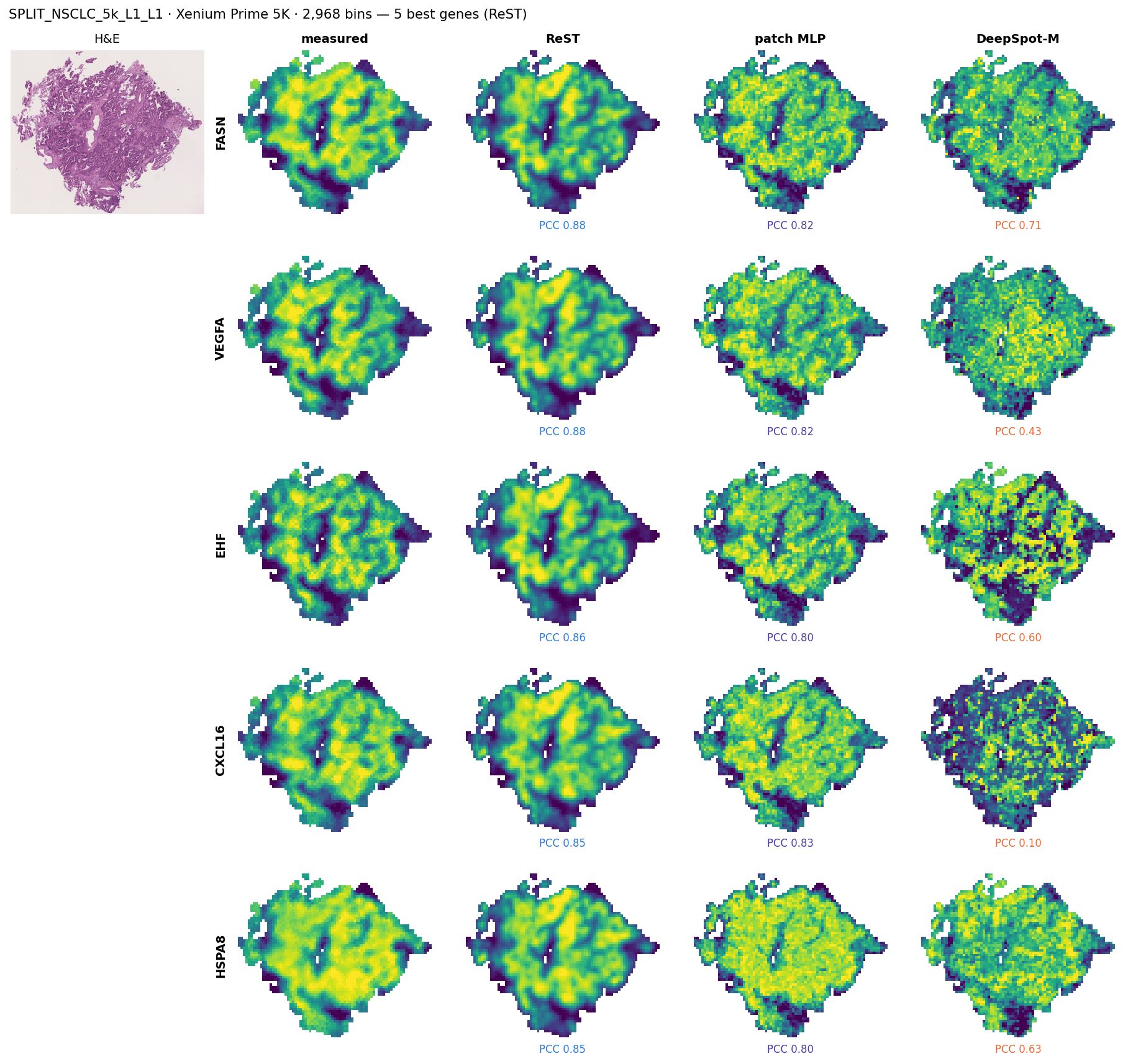
SPLIT_NSCLC_5k_L1_L1 (Xenium Prime 5K, median sample of its panel by ReST top-50): its 5 best genes for ReST, with the MLP and DeepSpot-M on the same genes.
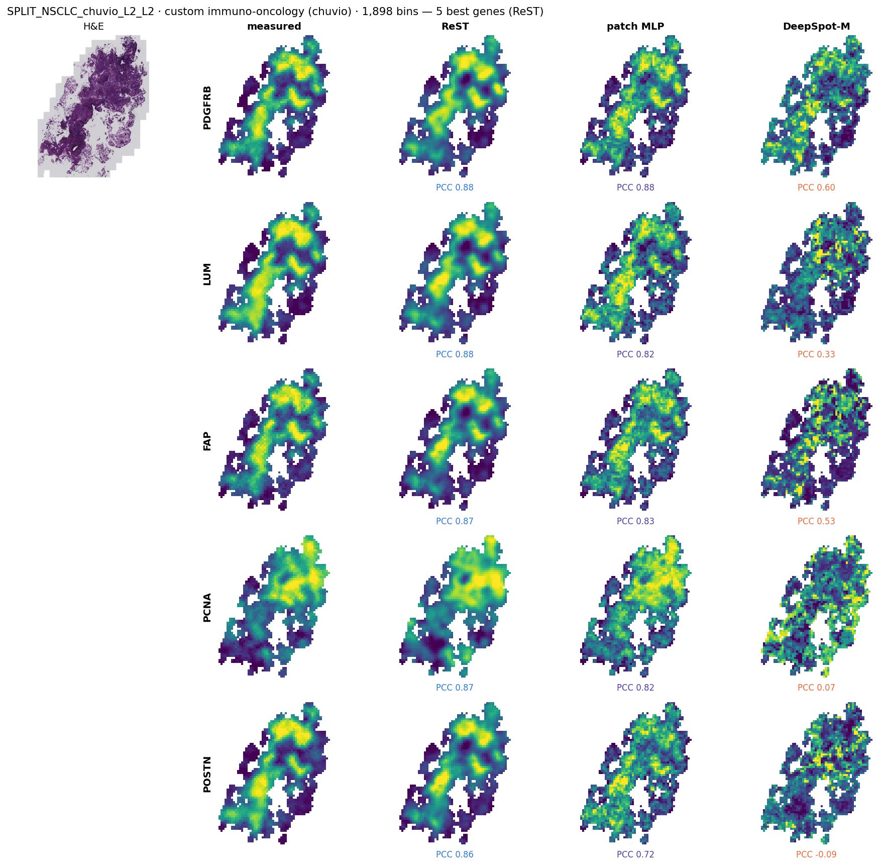
SPLIT_NSCLC_chuvio_L2_L2 (custom immuno-oncology (chuvio), median sample of its panel by ReST top-50): its 5 best genes for ReST, with the MLP and DeepSpot-M on the same genes.
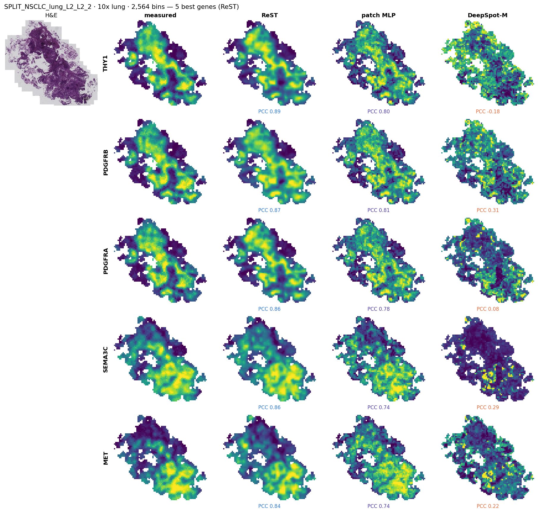
SPLIT_NSCLC_lung_L2_L2_2 (10x lung, median sample of its panel by ReST top-50): its 5 best genes for ReST, with the MLP and DeepSpot-M on the same genes.
New Xenium data, never seen by any model
Meninges, dura, fetal head and four new 10x slides: scored before any of them joins training
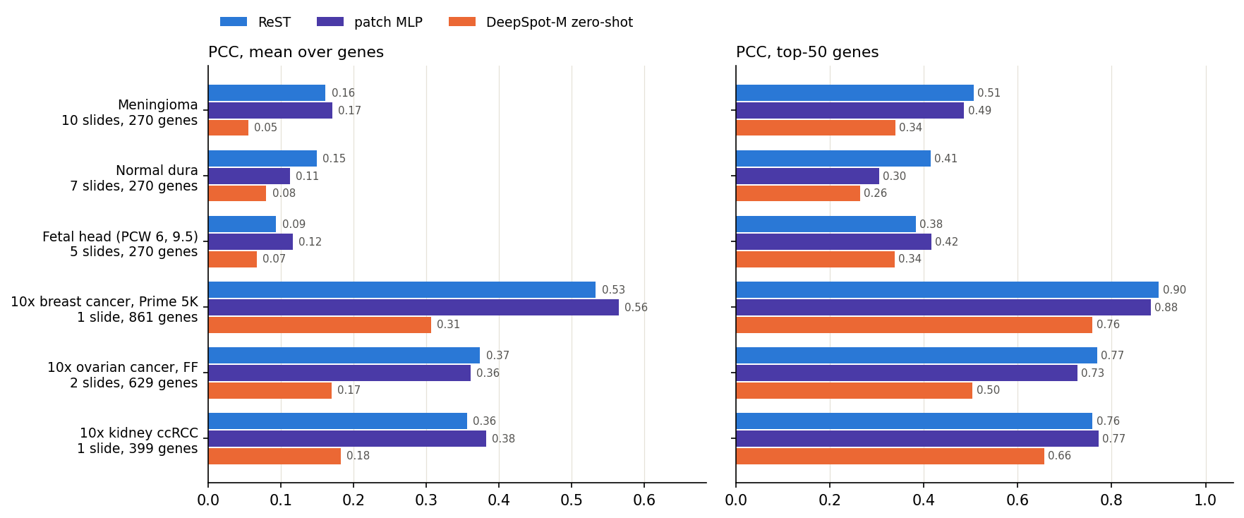
Mean over each group's slides of the per-slide mean / top-50 gene PCC (smoothed truth, 55 µm bins, the slide's measured genes in our panel).
data
Meninges atlas (BIA S-BIAD1600, CC0): 22 regions with post-Xenium H&E: meningioma (WHO 3 and 1), normal dura, fetal head; custom panel, 270 genes in ours
10x: breast Prime 5K, ovarian v1 + Prime 5K (fresh-frozen), kidney ccRCC; 399–861 genes in ours
Same 55 µm bins, 112 µm crops and truth as every other set; H&E registration checked per slide; bins kept only on stained tissue (as SPLIT)
reading
Best on top-50: ReST on meningioma, dura, 10x breast, 10x ovary; patch MLP on fetal head, 10x kidney
Best on mean: ReST on dura, 10x ovary; patch MLP on meningioma, fetal head, 10x breast, 10x kidney
New data: one slide per group
Click a group: H&E, measured, ReST, MLP and DeepSpot-M maps
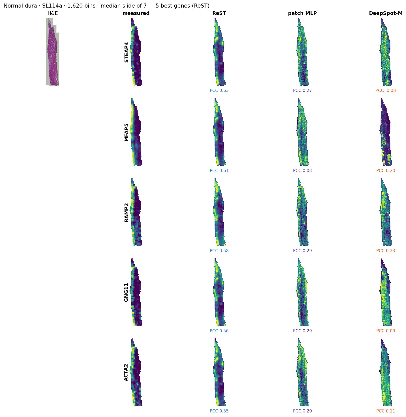
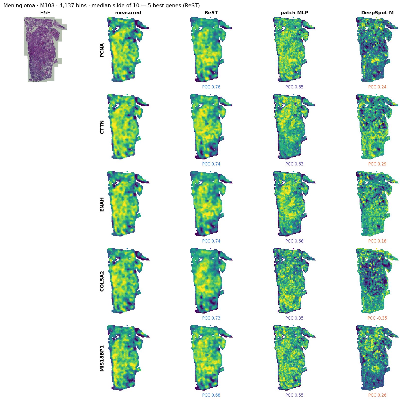
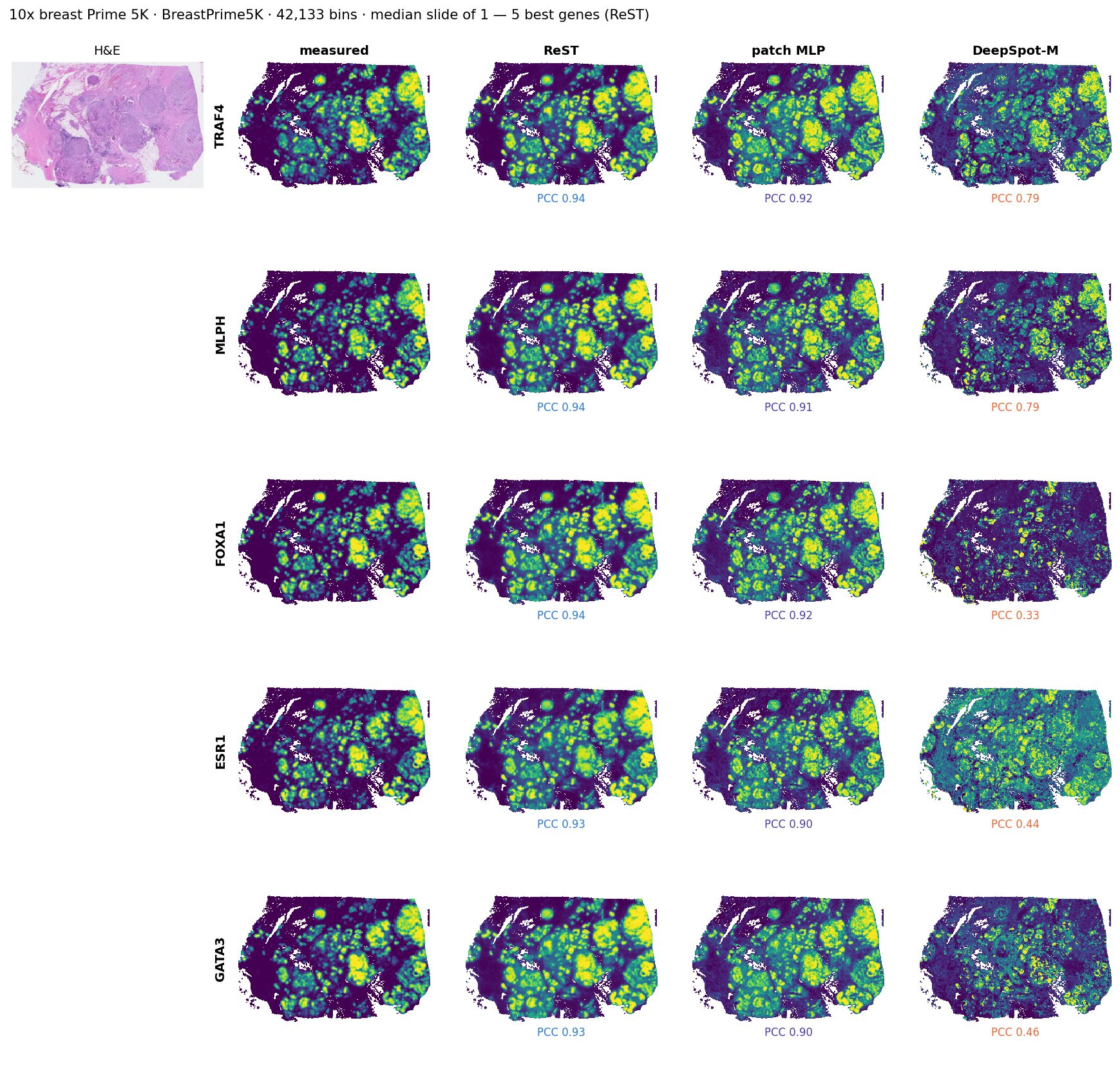
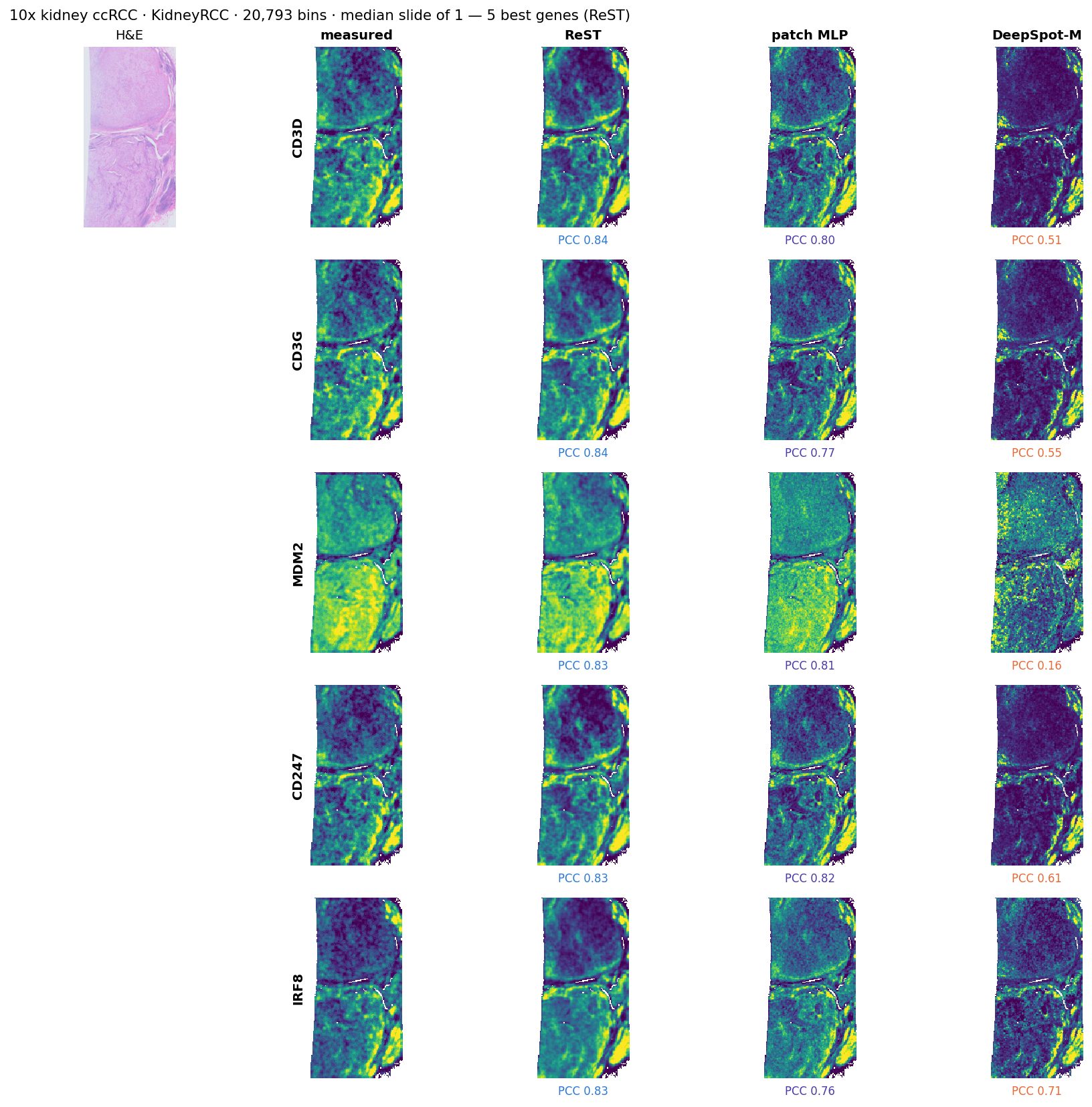
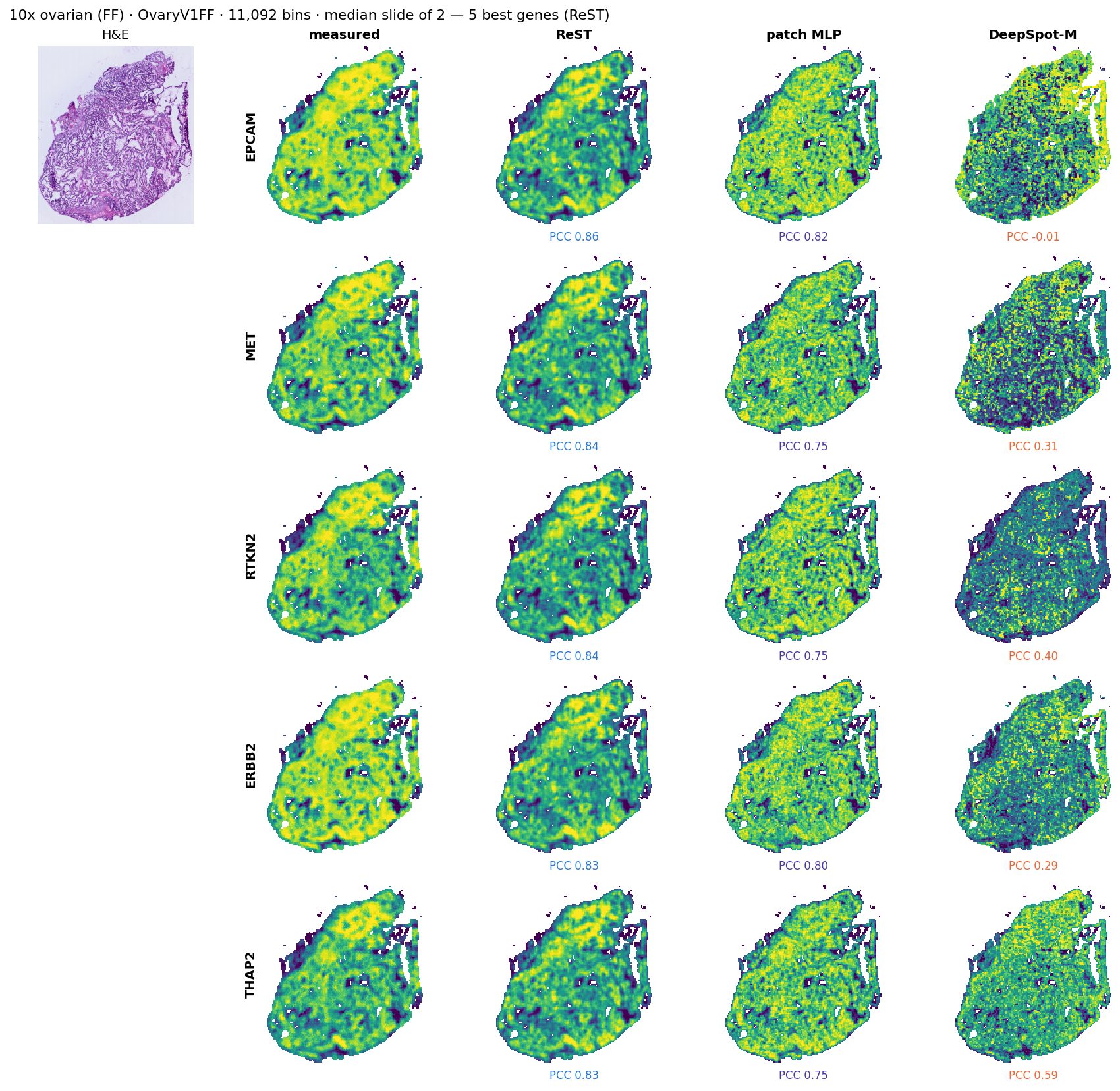
SL114a: the median slide of its group (7) by ReST top-50 PCC; its 5 best expressed genes for ReST, with the other models on the same genes. Each map scaled to its own 2nd–98th percentile.
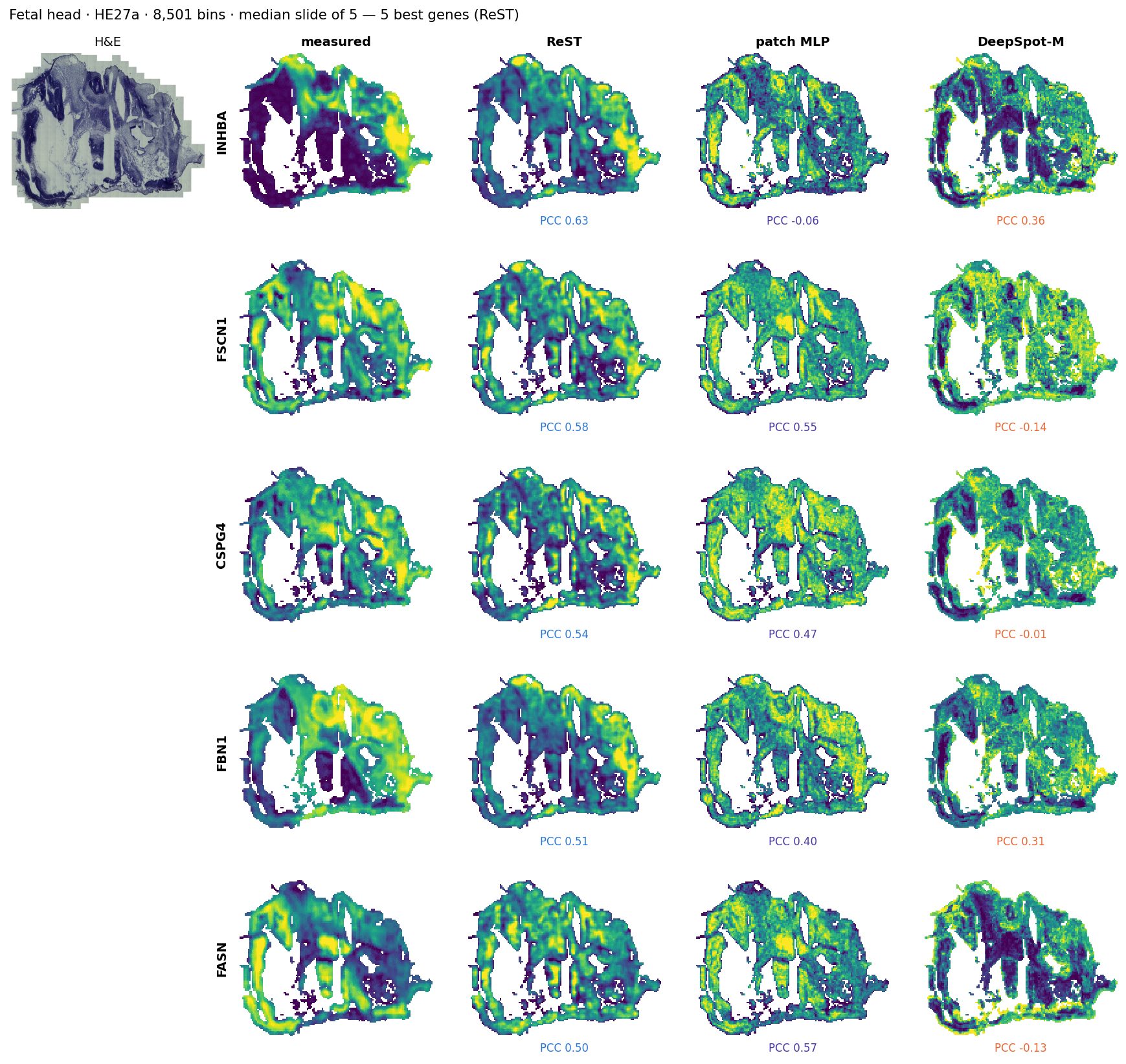
HE27a: the median slide of its group (5) by ReST top-50 PCC; its 5 best expressed genes for ReST, with the other models on the same genes. Each map scaled to its own 2nd–98th percentile.
M108: the median slide of its group (10) by ReST top-50 PCC; its 5 best expressed genes for ReST, with the other models on the same genes. Each map scaled to its own 2nd–98th percentile.
BreastPrime5K: the median slide of its group (1) by ReST top-50 PCC; its 5 best expressed genes for ReST, with the other models on the same genes. Each map scaled to its own 2nd–98th percentile.
KidneyRCC: the median slide of its group (1) by ReST top-50 PCC; its 5 best expressed genes for ReST, with the other models on the same genes. Each map scaled to its own 2nd–98th percentile.
OvaryV1FF: the median slide of its group (2) by ReST top-50 PCC; its 5 best expressed genes for ReST, with the other models on the same genes. Each map scaled to its own 2nd–98th percentile.
Instrument transfer: CosMx 6K, never seen by any model
Same H&E-to-expression task on a second imaging platform: CosMx 6K sections scored zero-shot
Per section: mean / top-50 gene PCC (smoothed truth, 55 µm bins on stained tissue, the section's genes in our panel). ReST and the MLP were trained on Xenium only, DeepSpot-M on Visium.
data
SPATCH (Ren et al., Nat Commun 2025): CosMx 6K whole sections of colon adenocarcinoma, liver cancer and ovarian cancer, H&E of the same section after the run
1083 panel genes in ours; 47,007 bins in total
Registration (none shipped): H&E = CosMx DAPI frame / 1.835; transcripts y-flipped and shifted 533 µm, found by cross-correlating transcript density with H&E (r = 0.38 vs ≤ 0.01 for other flips)
Binned, cropped and scored exactly as the Xenium sets
reading
Best on top-50: ReST on liver, ovary; zero-shot DeepSpot-M on colon
Best on mean: ReST on colon, ovary; patch MLP on liver
Same blocks on Xenium 5K (serial sections, SPATCH) would isolate the instrument; not downloaded yet
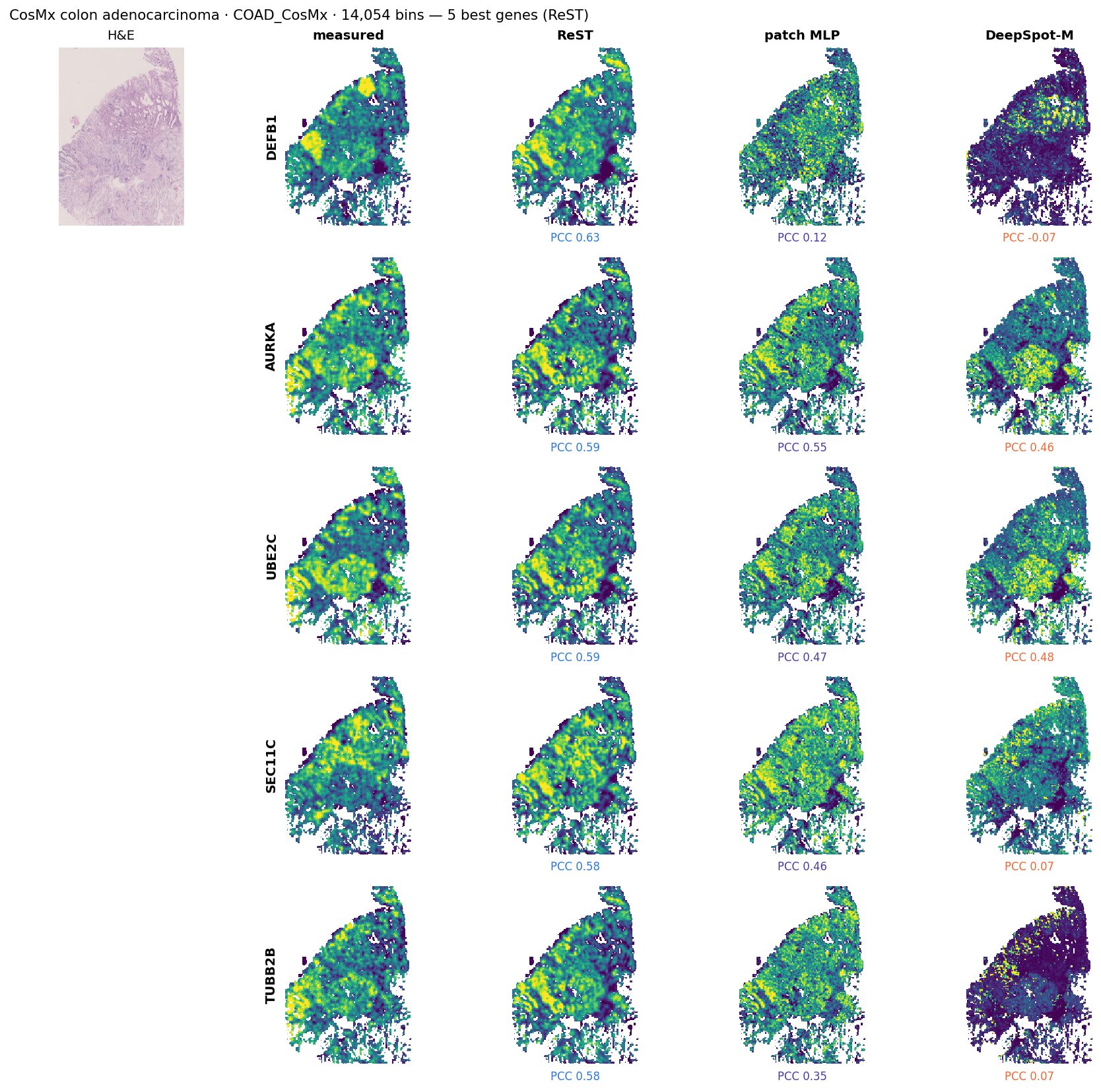
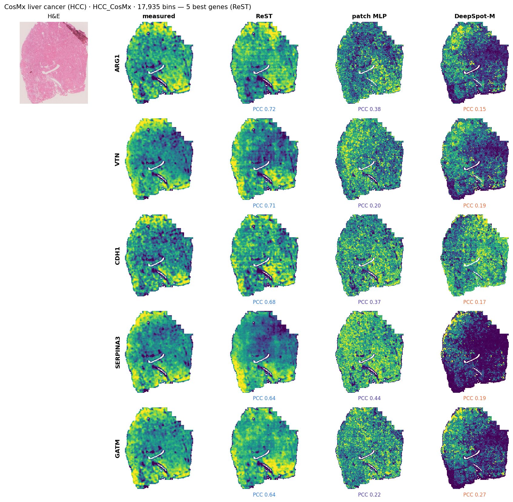
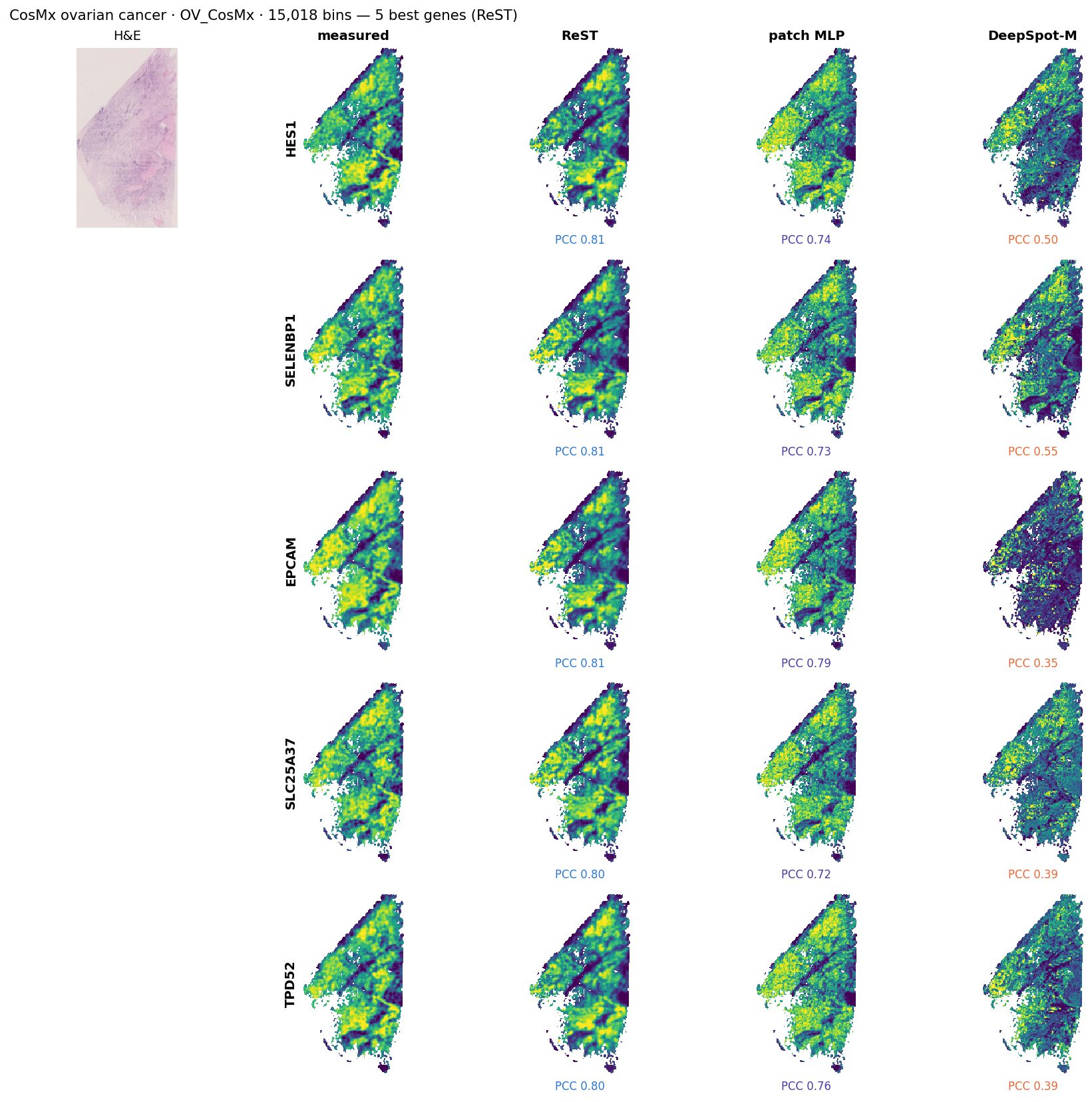
CosMx 6K: example maps
Click a tumour: H&E, measured (CosMx), ReST, MLP and DeepSpot-M maps
SPATCH_COAD_CosMx: its 5 best expressed genes for ReST, with the other models on the same genes. Each map scaled to its own 2nd–98th percentile.
SPATCH_HCC_CosMx: its 5 best expressed genes for ReST, with the other models on the same genes. Each map scaled to its own 2nd–98th percentile.
SPATCH_OV_CosMx: its 5 best expressed genes for ReST, with the other models on the same genes. Each map scaled to its own 2nd–98th percentile.
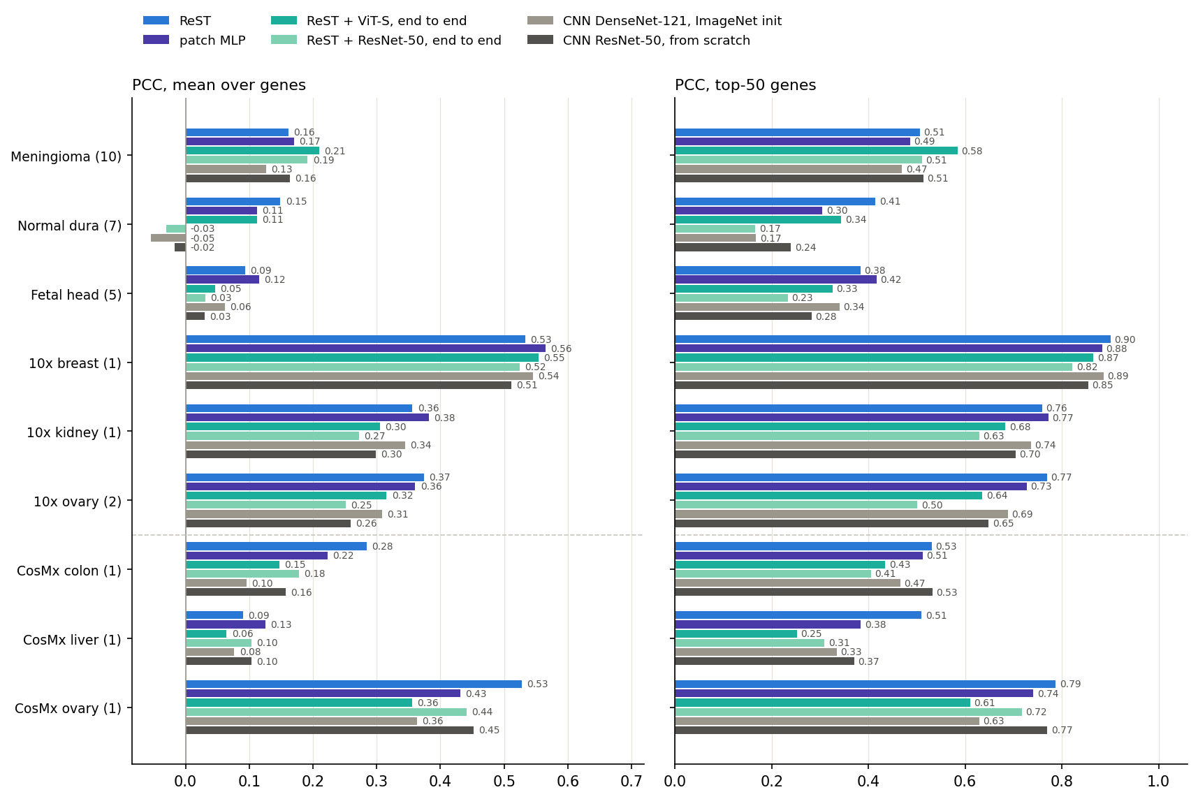
Without a foundation model: end to end
Pixels to genes without a pathology foundation model, per bin (CNN) and with slide context (ReST end to end)
Mean over each group's slides of the per-slide mean / top-50 gene PCC on data no model trained on (smoothed truth, same bins, genes and truth for every model). Above the dashed line: new Xenium data; below: CosMx 6K.
models
Input: the same 112 µm H&E crop per 55 µm bin, as pixels (224 px); no GigaPath features
CNN: per bin, trained end to end to the 1,622 genes on ReST's 68 training slides; ResNet-50 from scratch, DenseNet-121 from ImageNet weights (as ST-Net)
ReST end to end: an image encoder (ResNet-50 from the CNN above, or ViT-S/16 from ImageNet) in place of GigaPath, feeding the deck model's ReST trunk; both trained together on the same slides (k = 2, MSE + PCC loss)
ReST on GigaPath beats both end-to-end ReST models in 6 of 9 groups (not on Meningioma, 10x breast, CosMx liver)
ReST + ViT-S beats both per-bin CNNs in 4 of 9 groups
ResNet-50 encoders break on unfamiliar tissue (mean PCC): ReST + ResNet-50: Normal dura -0.03, Fetal head +0.03; CNN ResNet-50: Normal dura -0.02, Fetal head +0.03
The patch MLP on GigaPath features beats the from-scratch CNN in 8 of 9 groups
End to end vs GigaPath: the standard test sets
Same genes and bins as the deck's main comparisons
model
input
BEAT 108
10x test fold
unused HEST
liver
heart cores
old 10x
SPLIT
Visium
ReST (deck)
GigaPath
0.650 / 0.876
0.614 / 0.879
0.626 / 0.892
0.628 / 0.949
0.239 / 0.662
0.393 / 0.740
0.476 / 0.822
0.130 / 0.475
patch MLP
GigaPath
0.606 / 0.836
0.612 / 0.863
0.640 / 0.882
0.497 / 0.851
0.237 / 0.600
0.421 / 0.716
0.474 / 0.791
0.140 / 0.456
ReST + ViT-S e2e
pixels
0.545 / 0.797
0.607 / 0.856
0.627 / 0.885
0.554 / 0.923
0.247 / 0.644
0.400 / 0.684
0.416 / 0.765
0.120 / 0.441
ReST + ResNet-50 e2e
pixels
0.553 / 0.806
0.589 / 0.844
0.609 / 0.851
0.258 / 0.507
0.306 / 0.679
0.371 / 0.657
0.373 / 0.720
0.122 / 0.444
DenseNet-121 (ImageNet)
pixels
0.568 / 0.819
0.564 / 0.851
0.576 / 0.856
0.564 / 0.941
0.234 / 0.609
0.392 / 0.689
0.385 / 0.721
0.104 / 0.433
ResNet-50 (scratch)
pixels
0.552 / 0.811
0.549 / 0.841
0.550 / 0.833
0.573 / 0.928
0.247 / 0.607
0.337 / 0.635
0.317 / 0.679
0.101 / 0.424
Per-slide gene PCC, mean over genes / top-50 genes, averaged over slides; smoothed truth; all models on the same slides, bins and measured genes. Slides: BEAT 108 108 · 10x test fold 18 · unused HEST 29 · liver 1 · heart cores 195 · old 10x 3 · SPLIT 30 · Visium 98. Green: best per column.
reading
ReST on GigaPath leads every model trained on pixels in 5 of 8 sets on mean PCC and 7 of 8 on top-50 PCC
ReST + ViT-S end to end is within 0.01 mean PCC of it on 10x test fold, unused HEST, heart cores, old 10x, and falls behind on BEAT 108 (−0.105) and liver (−0.074)
The per-bin patch MLP on GigaPath, with no slide context, is at or above the best pixel model in 6 of 8 sets
Read-out on foundation-model features: GigaPath vs H-optimus-1
How much model the frozen features need, from one linear layer to slide-level recursion
model
features
val
BEAT 108
10x test fold
unused HEST
liver
heart cores
old 10x
SPLIT
Visium
ReST (deck)
GigaPath
0.666
0.650 / 0.876
0.614 / 0.879
0.626 / 0.892
0.628 / 0.949
0.239 / 0.662
0.393 / 0.740
0.476 / 0.822
0.130 / 0.475
ReST, FM-test recipe
GigaPath
0.626 / 0.931
0.627 / 0.864
0.592 / 0.863
0.603 / 0.876
0.599 / 0.943
0.261 / 0.665
0.366 / 0.720
0.443 / 0.809
0.134 / 0.495
patch MLP
GigaPath
0.665 / 0.926
0.606 / 0.835
0.610 / 0.859
0.640 / 0.882
0.525 / 0.874
0.232 / 0.590
0.421 / 0.715
0.467 / 0.782
0.136 / 0.449
linear probe
GigaPath
0.611 / 0.906
0.568 / 0.821
0.511 / 0.815
0.469 / 0.808
0.248 / 0.737
0.164 / 0.561
0.350 / 0.654
0.362 / 0.723
0.094 / 0.438
ReST, FM-test recipe
H-optimus-1
0.610 / 0.920
0.637 / 0.871
0.603 / 0.867
0.635 / 0.899
0.590 / 0.934
0.265 / 0.677
0.395 / 0.707
0.469 / 0.825
0.140 / 0.507
ReST, 5x input lr
GigaPath
0.639 / 0.939
0.637 / 0.871
0.603 / 0.877
0.614 / 0.886
0.612 / 0.947
0.266 / 0.672
0.384 / 0.732
0.462 / 0.823
0.142 / 0.512
ReST, 5x input lr
H-optimus-1
0.620 / 0.928
0.650 / 0.878
0.612 / 0.878
0.633 / 0.900
0.602 / 0.938
0.252 / 0.671
0.395 / 0.735
0.483 / 0.833
0.138 / 0.516
patch MLP
H-optimus-1
0.678 / 0.930
0.635 / 0.853
0.615 / 0.857
0.653 / 0.890
0.524 / 0.879
0.251 / 0.625
0.457 / 0.749
0.501 / 0.813
0.135 / 0.449
linear probe
H-optimus-1
0.615 / 0.903
0.598 / 0.841
0.521 / 0.825
0.484 / 0.824
0.247 / 0.744
0.181 / 0.588
0.357 / 0.687
0.425 / 0.764
0.104 / 0.455
Per-slide gene PCC, mean over genes / top-50 genes, averaged over slides; smoothed truth; same slides, bins and measured genes for every row. val: best validation epoch (ReST's 4 validation slides; mean / top-50). Patch MLP and linear probe: one 112 µm crop embedding per bin, no slide context, same training recipe (80 epochs, blank crops dropped, best validation epoch); the MLP has two hidden layers of 658. Green: best per column.
reading
The 2-layer MLP beats a single linear layer on the same GigaPath features in 8 of 8 sets, by 0.038–0.277 mean PCC: the features need a nonlinear read-out
ReST over the MLP: higher mean PCC in 5 of 8 sets, higher top-50 PCC in 8 of 8
ReST, FM-test recipe: H-optimus-1 minus GigaPath -0.009 to +0.033 mean PCC (higher in 7 of 8 sets)
ReST, 5x input lr: H-optimus-1 minus GigaPath -0.014 to +0.020 mean PCC (higher in 5 of 8 sets)
patch MLP: H-optimus-1 minus GigaPath -0.001 to +0.037 mean PCC (higher in 6 of 8 sets)
linear probe: H-optimus-1 minus GigaPath -0.001 to +0.063 mean PCC (higher in 7 of 8 sets)
The H-optimus-1 patch MLP, without slide context, against ReST on GigaPath (deck): higher mean PCC in 6 of 8 sets, higher top-50 PCC in 1 of 8
Recursion depth of the 50/50 mix
Test-time sweep of N_Z_H, N_Z_L and N_outer on one trained checkpoint, plus three trained depths
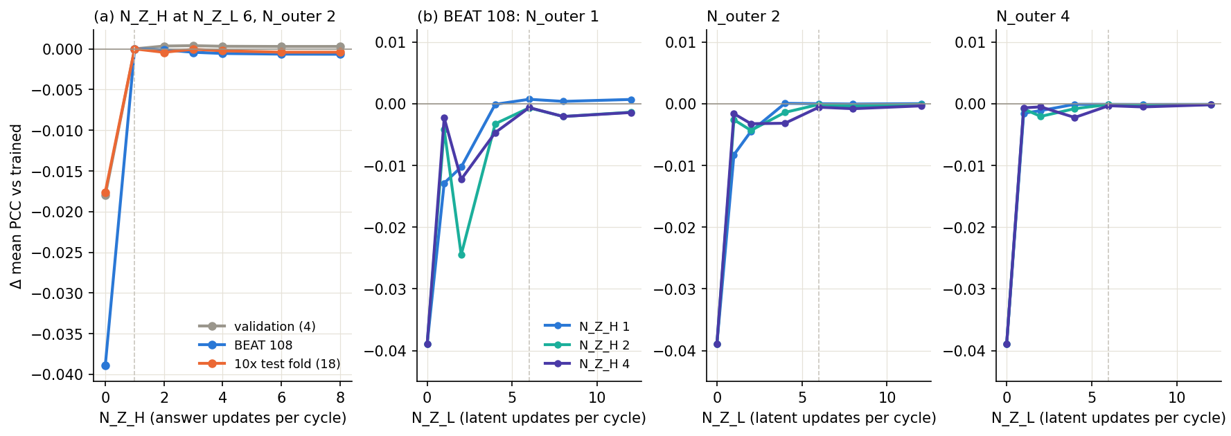
The trained trainable-mix checkpoint evaluated with other recursion counts. Change in mean per-gene PCC against the trained setting (N_Z_H 1, N_Z_L 6, N_outer 2; dashed lines). Per outer step: 3 cycles of N_Z_L latent updates, then N_Z_H answer updates.
reading
Removing the recursion's information (N_Z_L 0: the latent never updates, so the read-out never sees the slide) costs mean / top-50 PCC: BEAT 108 −0.039 / −0.037; 10x test fold −0.018 / −0.020; val −0.018 / −0.021
Depth saturates: from N_Z_L 4 on, every N_Z_H (1–4) and N_outer (1–4) is within 0.0047 mean PCC of the trained setting: extra test-time recursion neither helps nor hurts
One outer step suffices: N_outer 1 vs 2 at the trained N_Z_L / N_Z_H: BEAT 108 +0.0007; 10x test fold +0.0019; val +0.0003, at half the compute
Trained at other depths (2 epochs from the deck model, validation; control 0.6959): N_outer 1 0.6966 (+0.0007, 2 ep); N_Z_L 2 0.6948 (-0.0011, 2 ep); N_Z_H 2 0.6956 (-0.0003, 1 ep)
How FRM predicts a whole slide
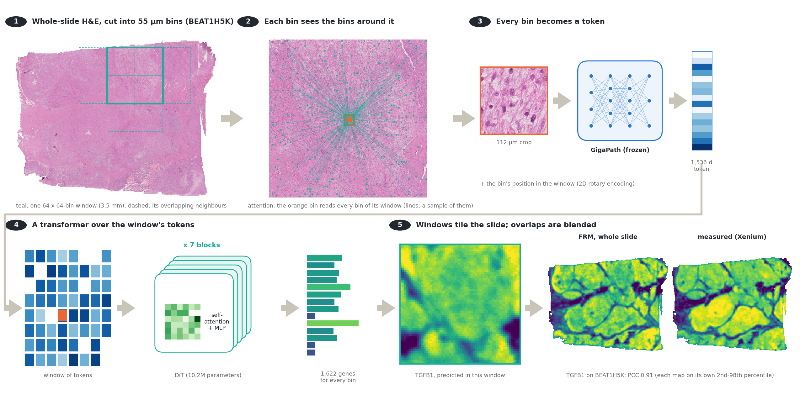
From an H&E slide to an expression map: bins, tokens, a transformer over each window, blended windows
Real data: BEAT1H5K (BEAT test set), the trained FRM (Fixed-Point Forcing checkpoint, t = 0 read-out). H&E shown in bin-grid space: each 55 µm bin's H&E, cut where its 112 µm crop was taken.
spatial context
A bin's prediction uses its own crop and every bin of its 3.5 mm window (up to 4,096 bins, ~1,000x the crop's area), through 7 rounds of self-attention; the patch MLP sees only the crop. Whole slide: windows at stride 32 bins, each bin in up to 4, Hann-weighted average
FRM: the network and the windows
A non-causal DiT over the bins of a 64 x 64-bin window, conditioned on GigaPath and on its own previous prediction
The trained FRM (Fixed-Point Forcing checkpoint) on validation slide TENX125. (1) windows assemble the slide; (2) inside a window, flow integration with the prediction fed back; (3) the read-out used, four refinements at t = 0. Gene SH2D3C is one of the best-predicted high-variance genes (slide PCC 0.97); most genes score lower (validation mean PCC about 0.71). Each map on its own 2nd–98th percentile. Play / pause: click the video.
Batch: 8 random 64 × 64-bin windows (ReST's 68 training slides, random view and flips)
Recipe: 40k steps, AdamW 3e-4, EMA; best of 20 validation checkpoints
windows vs whole slides
Windowed: a bin attends to the ≤ 4,096 bins of its 3.5 mm window
Whole-slide: a bin attends to the whole slide (as ReST), 2.5k + 2.5k steps
ReST: 2 shared blocks applied recursively over the whole slide
Flow Reasoning Models on the task
A self-conditioned flow over the expression map, with Fixed-Point Forcing, on GigaPath features
model
FRM — Helbling et al., arXiv 2026: a flow over the solution whose denoiser is fed its own previous prediction (self-conditioning), trained on its own rollouts (Fixed-Point Forcing)
Here: the solution is the expression map (1,622 genes per bin, standardised log1p); each bin's GigaPath embedding conditions it. xt = (1−t)ε + t y; a 7-block DiT (256 wide) predicts the clean map
Changed from the paper: MSE + PCC loss instead of cross-entropy (continuous outputs); training on 64 × 64-bin windows, whole slides by overlapping windows (or whole slides throughout, last two rows)
Samplers: t = 0 with 4 self-conditioned refinements (deterministic); Euler integration with self-conditioning, one sample or the mean of 4
arm
context
steps
t = 0, 4 refinements
Euler 8, 1 sample
Euler 8, mean of 4
Base flow (no self-conditioning)
64-bin windows
40,000 / 40,000
0.715 / 0.948
0.686 / 0.932
0.689 / 0.935
Stage A: + self-conditioning
64-bin windows
40,000 / 40,000
0.708 / 0.948
0.673 / 0.926
0.677 / 0.929
Stage B: self-conditioning only (control)
64-bin windows
18,000 / 40,000
0.708 / 0.948
0.673 / 0.927
0.677 / 0.930
Stage B: + Fixed-Point Forcing (FRM)
64-bin windows
14,000 / 40,000
0.710 / 0.948
0.674 / 0.928
0.678 / 0.931
Stage A: + self-conditioning
whole slides
2,500 / 2,500
0.554 / 0.866
0.624 / 0.904
0.625 / 0.905
Stage B: + Fixed-Point Forcing (FRM)
whole slides
2,500 / 2,500
0.597 / 0.888
0.654 / 0.920
0.656 / 0.921
Validation (ReST's 4 validation slides): mean / top-50 per-gene PCC, best checkpoint so far. For comparison on the same slides: deck ReST 0.666, patch MLP 0.665, trainable 50/50 mix 0.699. Test sets: next slide. Green: best per column.
reading
Best arm: Base flow (no self-conditioning) (64-bin windows), 0.715 validation mean PCC, above the 50/50 mix on these 4 slides
The deterministic t = 0 read-out beats integrating the flow late in training; the base flow is as good as self-conditioning and Fixed-Point Forcing adds little: the gain comes from the backbone (7 transformer blocks over many 64-bin windows), not the flow
Whole-slide training (2.5k steps of 4 slides) is far behind the windowed runs (40k steps of 8 windows)
FRM on the test sets
Same slides, bins and genes as every other model in the deck
model
context
BEAT 108
10x test fold
unused HEST
liver
heart cores
old 10x
SPLIT
Visium
FRM: base flow
windows
0.670 / 0.884
0.657 / 0.889
0.684 / 0.906
0.646 / 0.956
0.351 / 0.740
0.471 / 0.762
0.541 / 0.849
0.177 / 0.533
FRM: stage A, self-conditioning
windows
0.669 / 0.884
0.654 / 0.888
0.685 / 0.907
0.646 / 0.955
0.357 / 0.746
0.471 / 0.763
0.537 / 0.848
0.174 / 0.529
FRM: stage B, self-conditioning only
windows
0.669 / 0.884
0.654 / 0.888
0.685 / 0.908
0.647 / 0.955
0.359 / 0.747
0.470 / 0.762
0.536 / 0.847
0.173 / 0.528
FRM: stage B, Fixed-Point Forcing
windows
0.671 / 0.884
0.653 / 0.887
0.685 / 0.909
0.650 / 0.956
0.357 / 0.749
0.472 / 0.762
0.536 / 0.846
0.172 / 0.526
FRM: stage B, Fixed-Point Forcing
whole slides
0.592 / 0.817
0.609 / 0.850
0.634 / 0.865
0.574 / 0.918
0.269 / 0.619
0.422 / 0.673
0.470 / 0.778
0.143 / 0.439
same network as a plain regressor
windows
0.679 / 0.889
0.655 / 0.893
0.694 / 0.916
0.654 / 0.960
0.331 / 0.740
0.475 / 0.768
0.550 / 0.858
0.182 / 0.546
same network as a plain regressor, seed 1
windows
0.679 / 0.890
0.655 / 0.890
0.694 / 0.917
0.649 / 0.959
0.351 / 0.748
0.470 / 0.768
0.548 / 0.864
0.176 / 0.539
plain regressor, 128-bin windows
windows
0.682 / 0.889
0.659 / 0.892
0.686 / 0.911
0.651 / 0.958
0.322 / 0.732
0.472 / 0.760
0.525 / 0.845
0.168 / 0.527
plain regressor, no spatial context
one bin
0.619 / 0.839
0.622 / 0.866
0.661 / 0.892
0.628 / 0.950
0.251 / 0.600
0.435 / 0.715
0.475 / 0.790
0.136 / 0.446
plain regressor, width 512 (37M)
windows
0.679 / 0.890
0.653 / 0.889
0.690 / 0.911
0.653 / 0.960
0.348 / 0.748
0.475 / 0.767
0.546 / 0.858
0.179 / 0.541
plain regressor + multi-scale context (learned gate over bin / window / whole slide)
window + whole slide
0.680 / 0.888
0.656 / 0.891
0.695 / 0.915
0.649 / 0.957
0.339 / 0.733
0.476 / 0.766
0.549 / 0.858
0.182 / 0.549
FRM: base flow, 3 blocks (5.5M)
windows
0.668 / 0.883
0.657 / 0.889
0.689 / 0.914
0.644 / 0.954
0.334 / 0.722
0.473 / 0.763
0.538 / 0.848
0.179 / 0.535
FRM: base flow, 1 block (3.1M)
windows
0.656 / 0.874
0.652 / 0.884
0.687 / 0.913
0.640 / 0.954
0.302 / 0.706
0.469 / 0.757
0.520 / 0.840
0.166 / 0.515
ReST + patch MLP 50/50 (trainable)
whole slides
0.664 / 0.878
0.649 / 0.887
0.669 / 0.906
0.624 / 0.948
0.295 / 0.690
0.433 / 0.752
0.512 / 0.834
0.152 / 0.494
ReST (deck)
whole slides
0.650 / 0.876
0.614 / 0.879
0.626 / 0.892
0.628 / 0.949
0.239 / 0.662
0.393 / 0.740
0.476 / 0.822
0.130 / 0.475
patch MLP
one bin
0.606 / 0.835
0.610 / 0.859
0.640 / 0.882
0.525 / 0.874
0.232 / 0.590
0.421 / 0.715
0.467 / 0.782
0.136 / 0.449
Per-slide gene PCC, mean over genes / top-50 genes, averaged over slides; smoothed truth; same slides, bins and measured genes for every row. FRM rows: best validation checkpoint of each arm (stage B arms at 12k / 2k of 40k steps), read out with its best validation sampler (t = 0 refinement; whole slides: mean of 4 samples). Green: best per column. Expanded-cohort arms are left out: 23 of the 30 SPLIT samples are in their training or validation slides.
reading
The windowed FRM (base flow) beats the 50/50 mix in 8 of 8 sets on mean PCC (+0.006 to +0.055) and 7 of 8 on top-50; largest gains on heart cores +0.055, old 10x +0.038, SPLIT +0.030
The four windowed variants (no self-conditioning, self-conditioning, with or without Fixed-Point Forcing) agree within 0.008 mean PCC in every set: the flow recipe does not drive the gain
The same network trained as a plain regressor (no noise, no flow time) against the base flow: -0.020 to +0.009 mean PCC
Spatial context: the regressor on 64-bin windows against the same network with each bin attending only to itself: +0.026 to +0.080 mean PCC (+0.049 averaged over the sets)
Multi-scale context (whole slide pooled in 8- and 32-bin cells, per-bin learned gate) against the 64-bin regressor: -0.004 to +0.008 mean PCC (+0.001 averaged), although +0.008 on validation; regressor seed 0 vs seed 1: +0.000
Whole-slide training (2.5k + 2.5k steps of 4 slides) trails the windowed FRM by 0.029 to 0.088 mean PCC
FRM on BEAT 108: denoising steps and refinements
How the prediction depends on the number of network evaluations
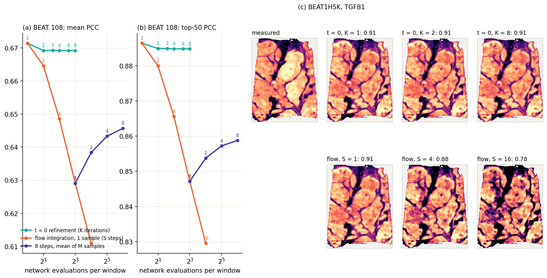
The trained FRM (Fixed-Point Forcing checkpoint) on every BEAT 108 slide with each read-out. (a, b) Mean over slides of the per-slide mean / top-50 gene PCC (smoothed truth) against network evaluations per window; numbers on the points: K, S or M. (c) One slide and gene, measured vs read-outs; each map on its own 2nd–98th percentile.
reading
t = 0 refinement: 0.671 after one pass, 0.669 after 4, 0.669 after 8 (mean PCC)
Flow integration (one sample): 0.671 with 1 step, 0.629 with 8, 0.611 with 16; averaging samples: 0.629 (1) to 0.646 (8 samples)
Best read-out on BEAT: a single pass at t = 0, 0.671 / 0.886 (the flow's first step is this same pass)
More flow steps lower the score: each sample carries noise, which per-gene PCC penalises; averaging samples recovers part of it. The prediction is the first deterministic pass, as for the plain-regressor control
Where FRM gains: genes
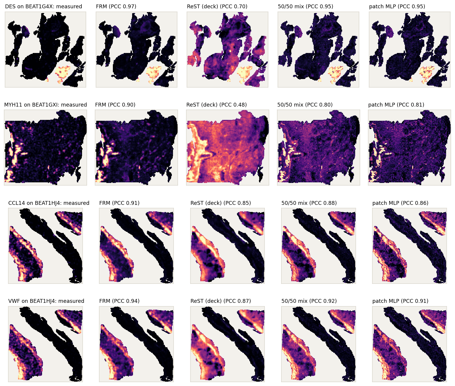
Per-gene PCC on BEAT 108, and the maps of the genes with the largest gain
The four genes with the largest FRM gain over the better of ReST (deck) and the patch MLP on BEAT 108 (mean over slides, table). Each is shown on the BEAT slide where FRM scores it highest (gene well expressed there), so the maps favour FRM; PCC of each map against the measured one. Each map on its own 2nd–98th percentile.
gene
FRM
ReST
MLP
gain
DES
0.408
0.269
0.275
+0.134
MYH11
0.562
0.318
0.443
+0.119
CCL14
0.683
0.589
0.593
+0.090
VWF
0.722
0.608
0.638
+0.084
LYVE1
0.515
0.439
0.416
+0.076
PLVAP
0.704
0.607
0.628
+0.076
S100B
0.586
0.502
0.510
+0.076
MCAM
0.675
0.587
0.606
+0.069
RGS5
0.674
0.607
0.603
+0.066
FLT1
0.663
0.586
0.598
+0.065
Mean over BEAT 108 slides of the per-slide gene PCC (smoothed truth); genes measured on ≥ 20 slides; gain over the better of ReST (deck) and the patch MLP.
reading
FRM beats both in 427 of 471 genes
The largest gains are smooth-muscle and vascular genes (DES, MYH11; VWF, PLVAP, MCAM, RGS5, LYVE1): thin structures such as vessel walls
Everything we tried: test sets
Scored on the held-out sets; fine-tunes start from ep29 / ep49 or the deck model
run
BEAT 108
10x test fold
SPLIT
Visium
BEAT vs ep29
Baselines
ReST ep29 (MSE, depth 8; starting point)
0.609 / 0.872
0.549 / 0.873
0.448 / 0.822
0.129 / 0.491
+0.000
patch MLP (per bin, GigaPath)
0.606 / 0.836
0.612 / 0.863
0.474 / 0.791
0.140 / 0.456
-0.003
DeepSpot-M, zero-shot
0.254 / 0.614
0.282 / 0.716
0.202 / 0.530
0.097 / 0.433
-0.355
ReST training
longer training: ep49 (MSE)
0.617 / 0.875
0.555 / 0.871
0.451 / 0.818
0.126 / 0.483
+0.008
fine-tune with a per-gene PCC loss
0.640 / 0.873
0.596 / 0.878
0.468 / 0.823
0.133 / 0.484
+0.031
PCC loss, depth 4
0.637 / 0.873
0.590 / 0.877
0.465 / 0.823
0.133 / 0.486
+0.028
+ rare-gene PCC weighting
0.641 / 0.873
0.599 / 0.878
0.470 / 0.823
0.134 / 0.485
+0.032
+ slide distribution losses
0.621 / 0.870
0.562 / 0.872
0.451 / 0.815
0.129 / 0.484
+0.012
+ distribution losses, 3× weight
0.609 / 0.868
0.551 / 0.869
0.444 / 0.811
0.126 / 0.482
+0.000
PCC + rare, depth 2 (grogu)
0.647 / 0.876
–
0.470 / 0.819
–
+0.038
PCC + rare, depth 4 (grogu)
0.647 / 0.876
–
0.469 / 0.818
–
+0.038
PCC + rare, depth 8 (grogu)
0.642 / 0.876
–
0.464 / 0.819
–
+0.033
+ spread (variance) loss, depth 4
0.647 / 0.876
–
0.469 / 0.818
–
+0.038
per-gene halting, depth 4 (deck model)
0.650 / 0.876
0.614 / 0.879
0.476 / 0.822
0.130 / 0.475
+0.041
ReST + patch MLP
MLP path + recursion, trainable MLP, depth 4
0.630 / 0.844
–
0.487 / 0.797
–
+0.021
MLP path + recursion, frozen MLP, depth 4
0.621 / 0.839
–
0.478 / 0.788
–
+0.012
average of deck model and MLP predictions
0.659 / 0.876
–
0.513 / 0.838
–
+0.050
trained 50/50 ReST + MLP mix, trainable MLP
0.664 / 0.878
0.649 / 0.887
0.512 / 0.834
0.152 / 0.494
+0.055
trained 50/50 mix, frozen MLP
0.662 / 0.877
0.645 / 0.885
0.507 / 0.831
0.150 / 0.490
+0.053
Without GigaPath
CNN ResNet-50, from scratch
0.552 / 0.811
0.549 / 0.841
0.317 / 0.679
0.101 / 0.424
-0.057
CNN DenseNet-121, ImageNet weights
0.568 / 0.819
0.564 / 0.851
0.385 / 0.721
0.104 / 0.433
-0.041
ReST + ViT-S, end to end
0.545 / 0.797
0.607 / 0.856
0.416 / 0.765
0.120 / 0.441
-0.064
ReST + ResNet-50, end to end
0.553 / 0.806
0.589 / 0.844
0.373 / 0.720
0.122 / 0.444
-0.056
Read-out
linear probe on GigaPath
0.568 / 0.821
0.511 / 0.815
0.362 / 0.723
0.094 / 0.438
-0.041
Flow Reasoning Model
FRM base flow, 64-bin windows
0.670 / 0.884
0.657 / 0.889
0.541 / 0.849
0.177 / 0.533
+0.061
FRM + Fixed-Point Forcing, 64-bin windows
0.671 / 0.884
0.653 / 0.887
0.536 / 0.846
0.172 / 0.526
+0.062
FRM + Fixed-Point Forcing, whole slides
0.592 / 0.817
0.609 / 0.850
0.470 / 0.778
0.143 / 0.439
-0.017
Per-slide gene PCC, mean over genes / top-50 genes, averaged over slides; smoothed truth; same slides, bins and genes per set. –: set not scored for that run. Last column: change in BEAT mean PCC against ReST ep29. Green: best per column.
Everything we tried: validation runs on grogu
One A6000 per run; the test-set scores of the main ones are on the previous slide
run
val (best epoch)
epochs
Round 1
depth 2, PCC + rare-gene PCC
0.658 / 0.945
2
depth 4, PCC
0.646 / 0.945
1
depth 4, PCC + rare
0.650 / 0.945
1
depth 4, + spread loss
0.650 / 0.945
1
Round 2
per-gene halting, depth 4 (deck model)
0.666 / 0.947
1
per-slide halting, depth 4
0.654 / 0.946
1
MLP path + recursion, trainable MLP, depth 4
0.678 / 0.930
1
same, frozen MLP
0.674 / 0.928
2
Round 3
per-gene halting, depth 2
0.660 / 0.946
1
MLP path + recursion, depth 2
0.678 / 0.930
1
same, frozen MLP
0.673 / 0.927
1
depth 2, one more epoch
0.661 / 0.946
1
Round 4
per-gene halting, depth 2, halting temperature 0.5
0.659 / 0.945
1
depth 2, 1 slide per step, PCC
0.651 / 0.945
1
depth 2, 1 slide per step, PCC + rare
0.656 / 0.945
1
Round 5
depth 2, 1 slide per step, PCC + rare, seed 0
0.668 / 0.945
4
same, seed 1
0.668 / 0.946
4
same, seed 2
0.668 / 0.946
4
same, rare-gene weight 1.0
0.671 / 0.945
4
depth 2, 4 slides per step, PCC + rare
0.666 / 0.946
4
depth 4, 1 slide per step, PCC + rare
0.665 / 0.945
3
low-rank gene-embedding output head
0.632 / 0.941
2
run
val (best epoch)
epochs
Round 5
trained on unsmoothed targets †
0.644 / 0.931
2
MLP path + recursion, depth 2
0.684 / 0.933
3
50/50 ReST + MLP mix, trainable MLP
0.696 / 0.949
2
50/50 mix, frozen MLP
0.695 / 0.949
3
same, seed 1
0.692 / 0.949
1
frozen mix, MLP share 0.4
0.691 / 0.950
1
frozen mix, MLP share 0.6
0.693 / 0.947
1
Round 6
continue the round-5 trainable 50/50 mix
0.698 / 0.950
4 of 4
50/50 mix, 6-epoch schedule
0.699 / 0.950
5 of 6
same, frozen MLP
0.697 / 0.949
5 of 6
50/50 mix, depth 4
0.697 / 0.950
2 of 3
same, frozen MLP
0.695 / 0.949
2 of 3
50/50 mix, expanded cohort ‡
0.636 / 0.914
4 of 4
same, frozen MLP ‡
0.625 / 0.908
4 of 4
plain ReST, expanded cohort ‡
0.618 / 0.912
4 of 4
trainable mix, seed 1, 1 epoch
0.693 / 0.949
1 of 1
Round 7
trainable mix, N_outer 1
0.697 / 0.950
2 of 2
trainable mix, N_Z_L 2
0.695 / 0.948
2 of 2
trainable mix, N_Z_H 2
0.696 / 0.950
1 of 2
expanded-cohort mix continued ‡
0.637 / 0.915
1 of 2
expanded-cohort plain ReST continued ‡
0.619 / 0.912
1 of 2
works
50/50 mix of ReST and the patch MLP: best run on both metrics (0.696 / 0.949 vs plain ReST 0.668 / 0.945); trainable or frozen MLP, MLP share 0.4–0.6 and seeds all within 0.005
Per-gene halting at depth 4: 0.666 vs per-slide halting 0.654 and fixed depth 4 0.650
MLP path + recursion (no mixing): mean 0.684 (+0.016) but top-50 0.933 (-0.012); the 50/50 mix keeps both
no gain
Recursion depth beyond 2: depth 4 0.665 vs depth 2 0.668 (3 seeds, range 0.0003)
Slides per step: 4 vs 1: 0.666 vs 0.668
Spread (variance) loss: 0.650 vs 0.650 without; slide distribution losses lowered the test scores (previous slide)
Low-rank gene-embedding head: 0.632 (-0.036)
More epochs of the mix (round 6, so far): 0.698 vs 0.696, within seed range
Mean / top-50 gene PCC on ReST's 4 validation slides (smoothed truth), best epoch. Fine-tunes on one A6000 each, from ep49 (rounds 1–5) or the deck model (mix runs); PCC loss weight 0.5 throughout. † validated against unsmoothed truth, not comparable. ‡ expanded cohort (111 training slides incl. the 2026-10 Xenium data), validated on its 8 validation slides, not comparable with the rest. Round 7 still running. Green: best comparable run.
Why did ReST ep29 trail the patch MLP on mean PCC?
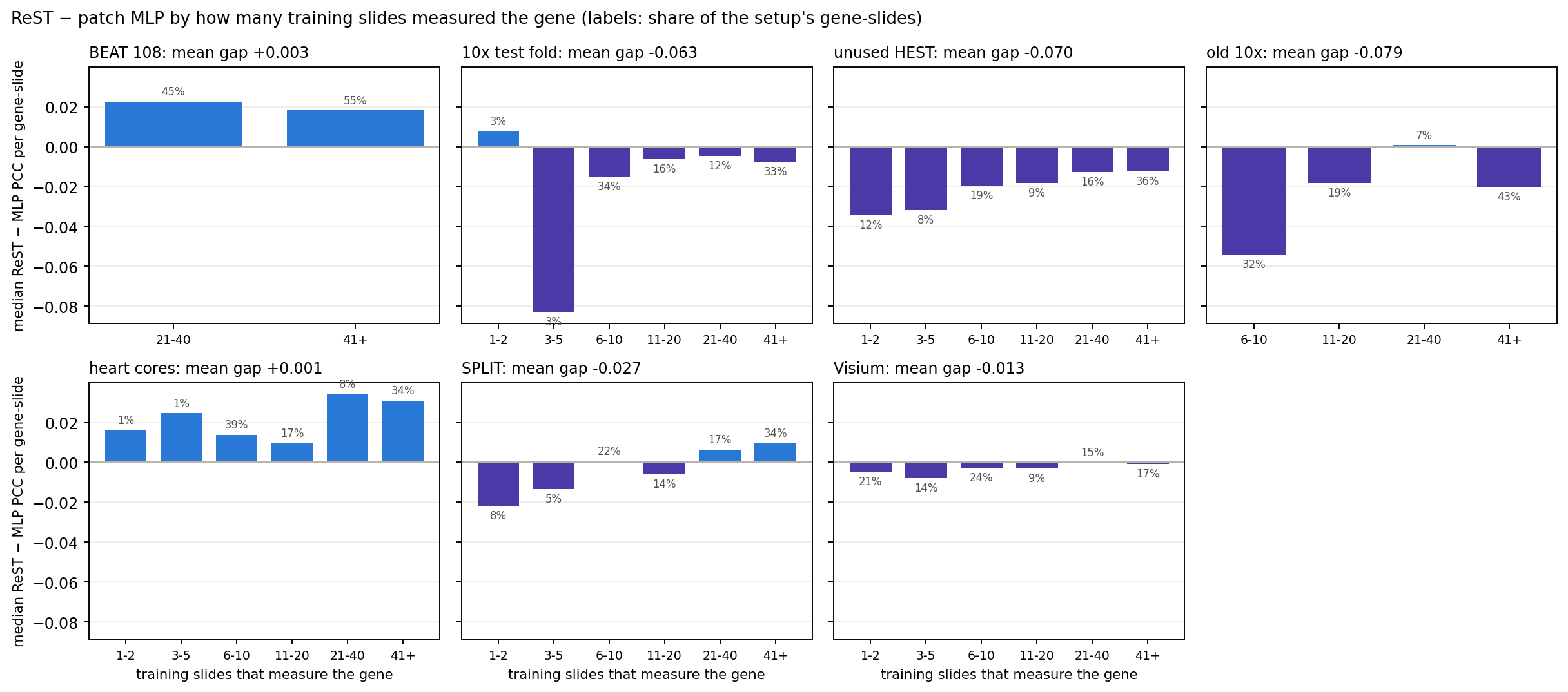
Test: is the MLP's lead carried by genes measured on few training slides?
hypothesis
ReST ep29 (MSE only); this analysis led to the deck’s PCC fine-tune. ReST trains on one whole slide per step, so a gene measured on few training slides gives it few examples.
The patch MLP sees every bin of those slides as a separate example.
training coverage
68 training slides; the median gene is measured on 9
339 of 1,622 genes are on only 1–2 slides
Genes on 1–5 slides are 6% of 10x-test gene-slides, 20% of unused HEST, 13% of SPLIT, 0% of BEAT
reading the bars
Where the MLP leads (10x, unused HEST, old 10x), it also leads on genes measured on 41+ training slides; those genes are mostly sparse on the test slides (see "are the well-covered genes sparse?").
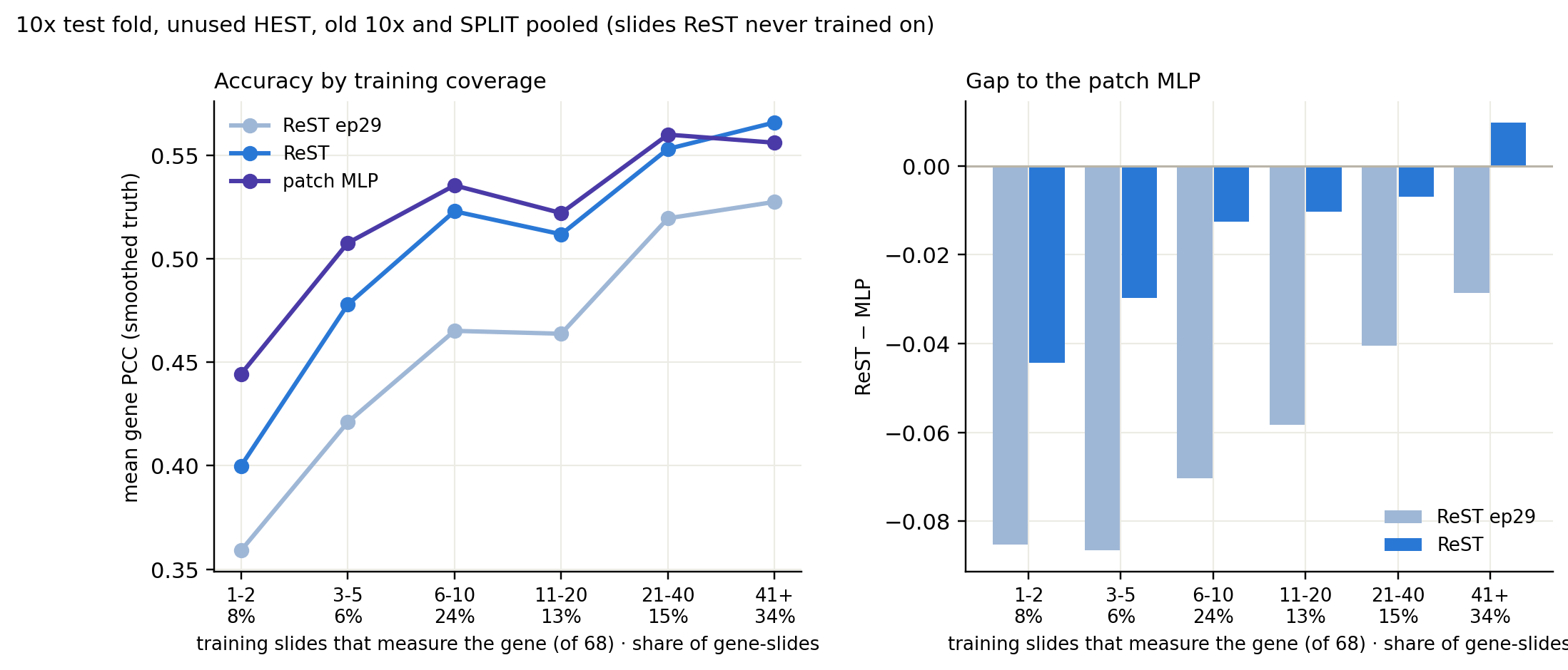
Median ReST − MLP PCC per gene-slide, binned by how many training slides measure the gene. Blue: ReST higher; purple: MLP higher. Labels: share of the setup's gene-slides.
MLP gap: coverage vs expression
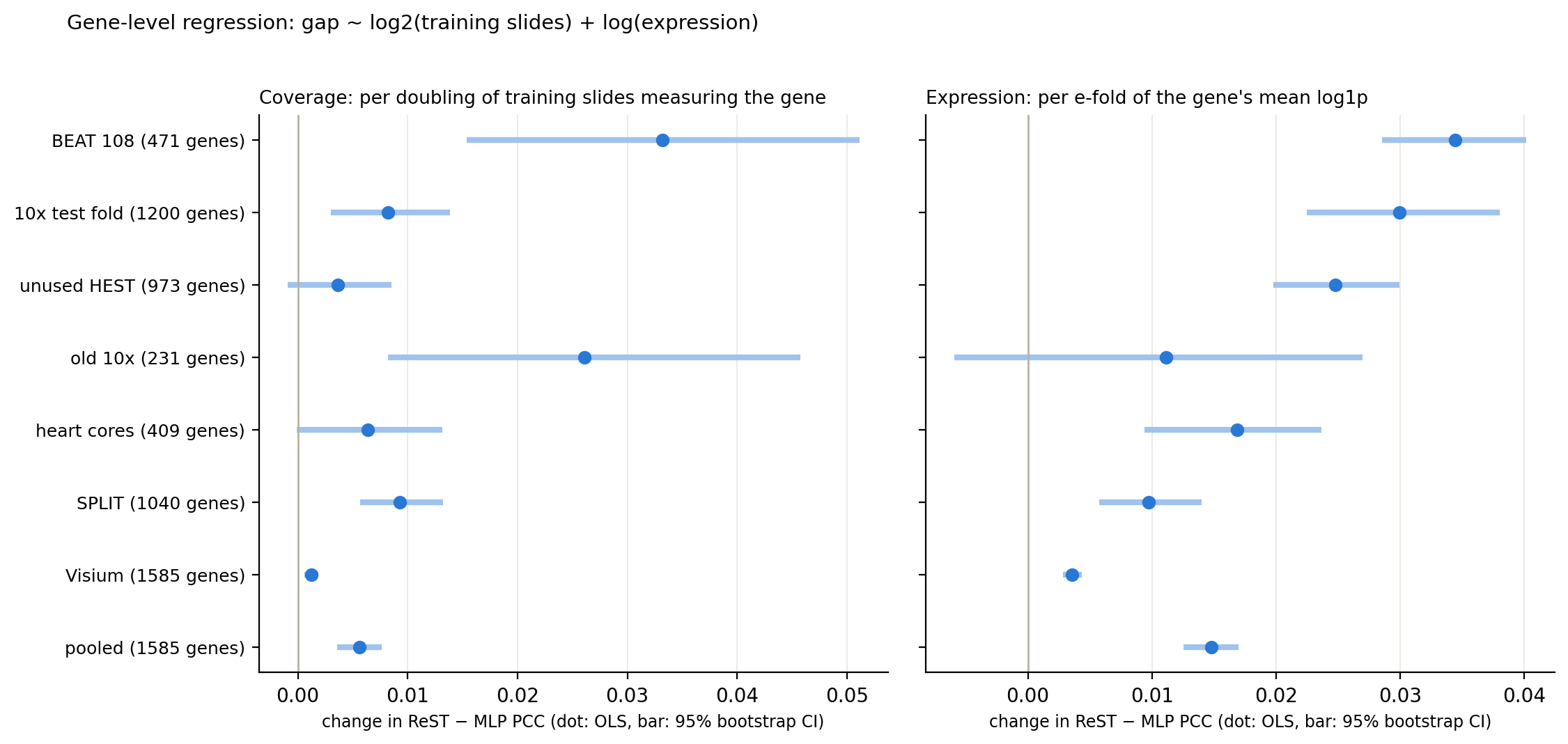
Gene-level regression: both coverage and expression predict the gap; expression has the larger effect
One row per gene (median gap over the setup's slides). Pooled: setup fixed effects; CIs from 2,000 bootstrap resamples of genes.
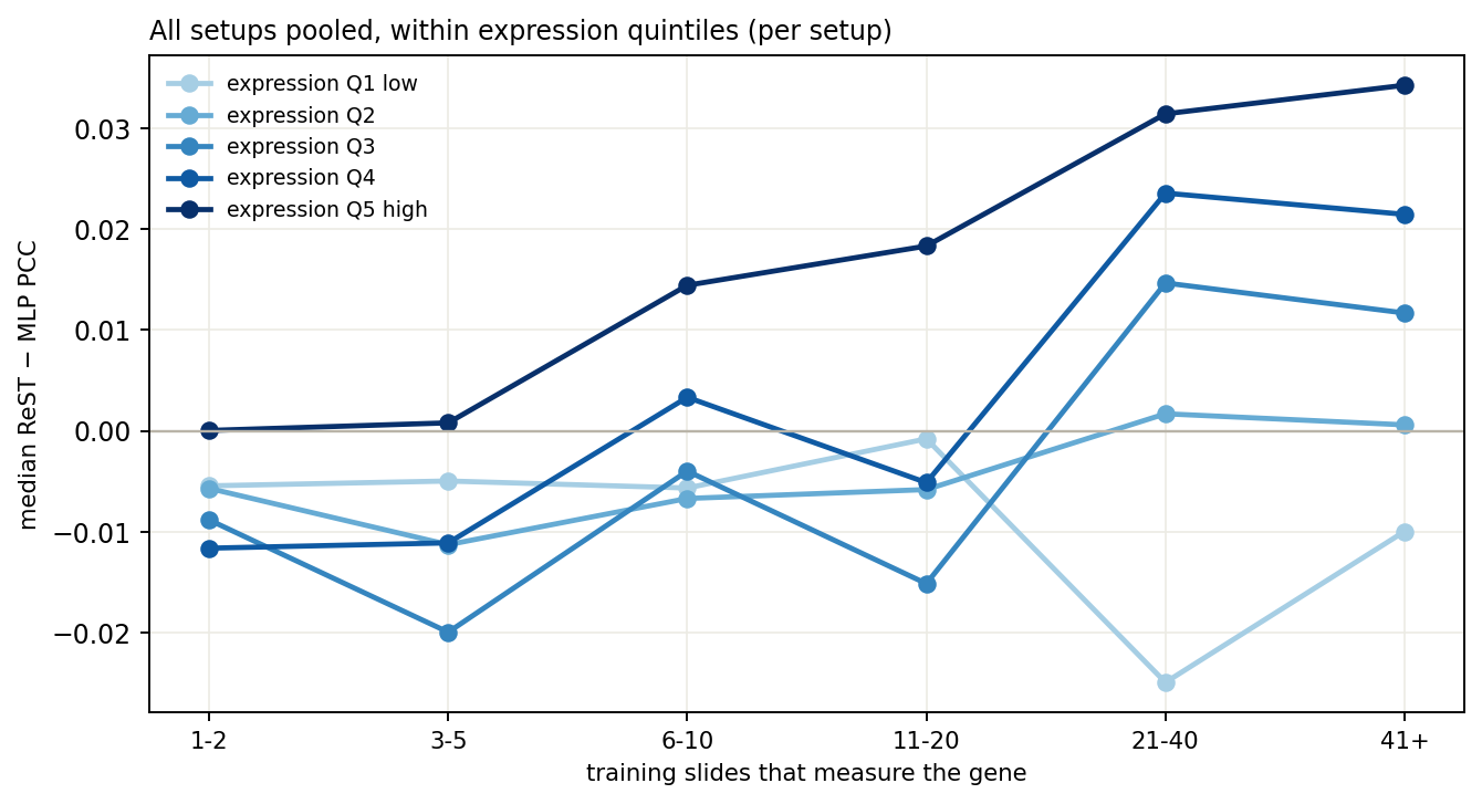
All setups pooled; expression quintiles taken within each setup.
+0.0056
pooled gap change per doubling of training slides (95% CI 0.0036–0.0076)
+0.0148
pooled gap change per e-fold of expression (95% CI 0.0126–0.0170)
Coverage matters: the gap moves toward ReST with more training slides in 5 of 7 setups (CI above 0); not in unused HEST or heart cores
Expression matters more: from 2 to 64 training slides moves the gap by 0.028; a 10× rise in expression moves it by 0.034
Coverage given expression (partial Spearman): 0.04–0.15 — weak
Low-expression genes favour the MLP at every coverage; highly expressed genes on 21+ slides favour ReST
MLP gap: dropping rarely measured genes
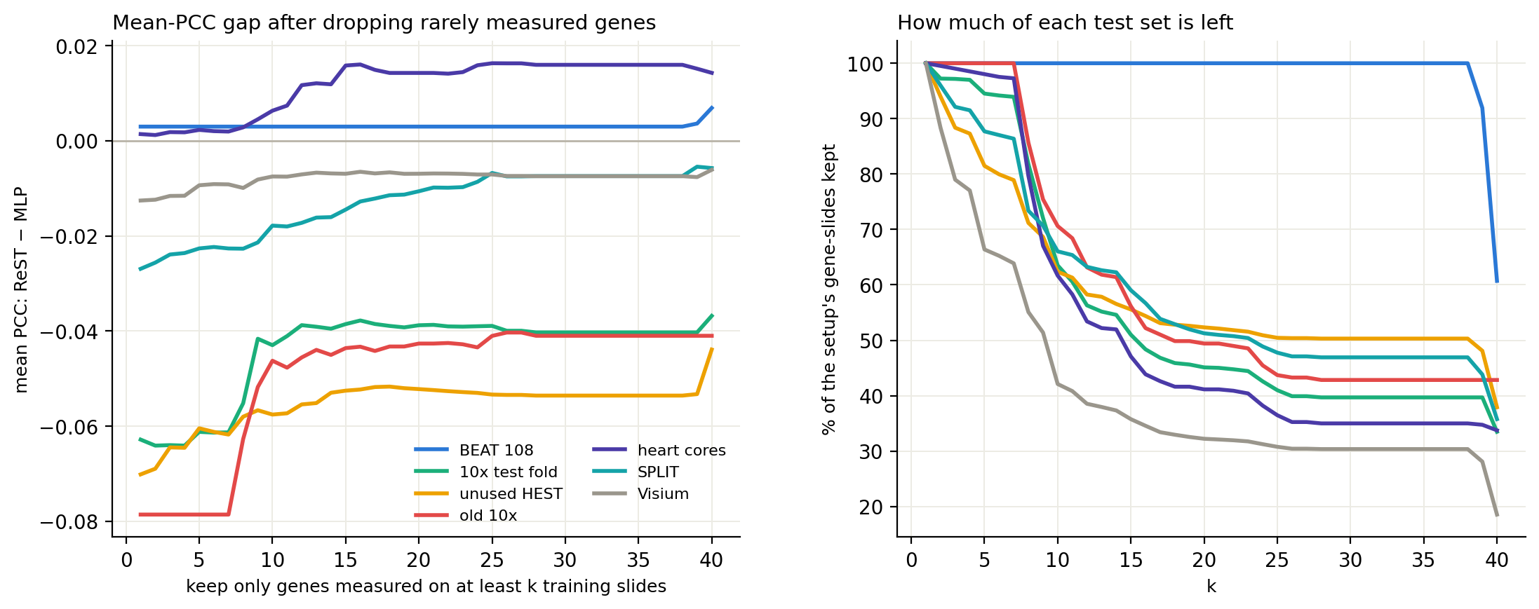
Rare genes explain part of the MLP's lead, not all of it: on well-measured 10x and HEST genes the MLP still leads by 0.04–0.05
Left: mean PCC gap over gene-slides of genes measured on at least k training slides. Right: share of each test set left.
-0.063 → -0.039
10x test fold, k = 1 → 21 (45% of gene-slides left)
-0.070 → -0.052
unused HEST (52% left)
-0.079 → -0.043
old 10x (49% left)
-0.027 → -0.010
SPLIT (51% left)
25–63%
of the MLP's lead removed by keeping genes on ≥ 21 training slides
MLP gap: are the well-covered genes sparse?
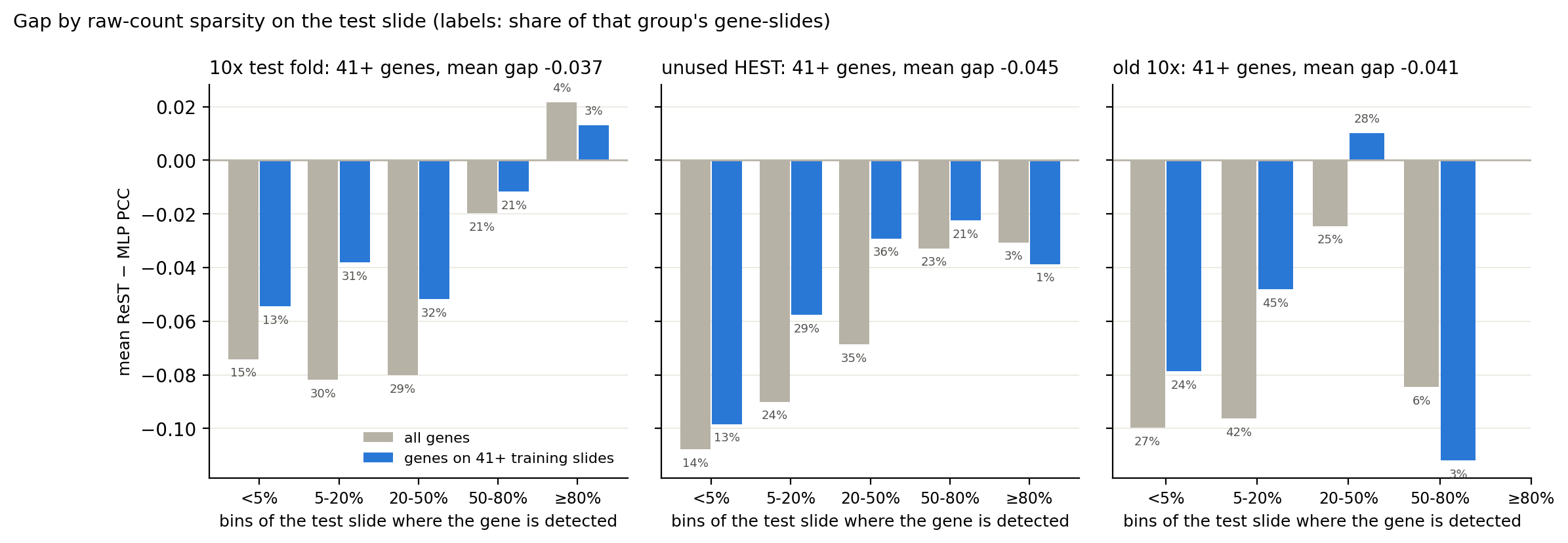
Mostly yes: the median well-covered gene is detected in 10–26% of bins, and the MLP's lead is largest where genes are sparsest
Raw counts in the same 55 µm bins as the caches (no smoothing). Grey: all genes; blue: genes on 41+ training slides.
Genes on 41+ training slides are sparse on these test slides: the median one is detected in 25% of bins (10x test), 26% (unused HEST), 10% (old 10x), with 0.53, 0.75 and 0.14 transcripts per bin
In unused HEST and old 10x the MLP's lead on these genes sits in the sparse gene-slides; in the 10x test fold it is nearly as large on genes detected in 20–50% of bins
Detected in ≥50% of bins: 24% / 22% / 3% of these gene-slides, gap -0.008 / -0.023 / -0.112 (10x test / unused HEST / old 10x; old 10x: 9 gene-slides)
-0.043 vs -0.033
10x test fold: gap where the gene is detected in <20% vs ≥20% of bins (44% / 56% of gene-slides)
-0.071 vs -0.027
unused HEST: gap where the gene is detected in <20% vs ≥20% of bins (42% / 58% of gene-slides)
-0.059 vs -0.002
old 10x: gap where the gene is detected in <20% vs ≥20% of bins (69% / 31% of gene-slides)
MLP gap: how much comes from sparse or rarely trained genes
Sparse or rarely trained genes carry 86–98% of the MLP's lead; dense genes seen on 21+ training slides add less than 0.01 to it
Each gene-slide falls in one group: sparse = detected in <20% of the test slide's bins (raw counts); rare = on <21 of the 68 training slides. Bars: each group's share of the total gap.
10x test fold, unused HEST and old 10x pooled.
86%
of the 10x test fold gap (-0.063) is on sparse or rarely trained genes; dense, common genes: -0.009
87%
of the unused HEST gap (-0.071) is on sparse or rarely trained genes; dense, common genes: -0.009
98%
of the old 10x gap (-0.080) is on sparse or rarely trained genes; dense, common genes: -0.002
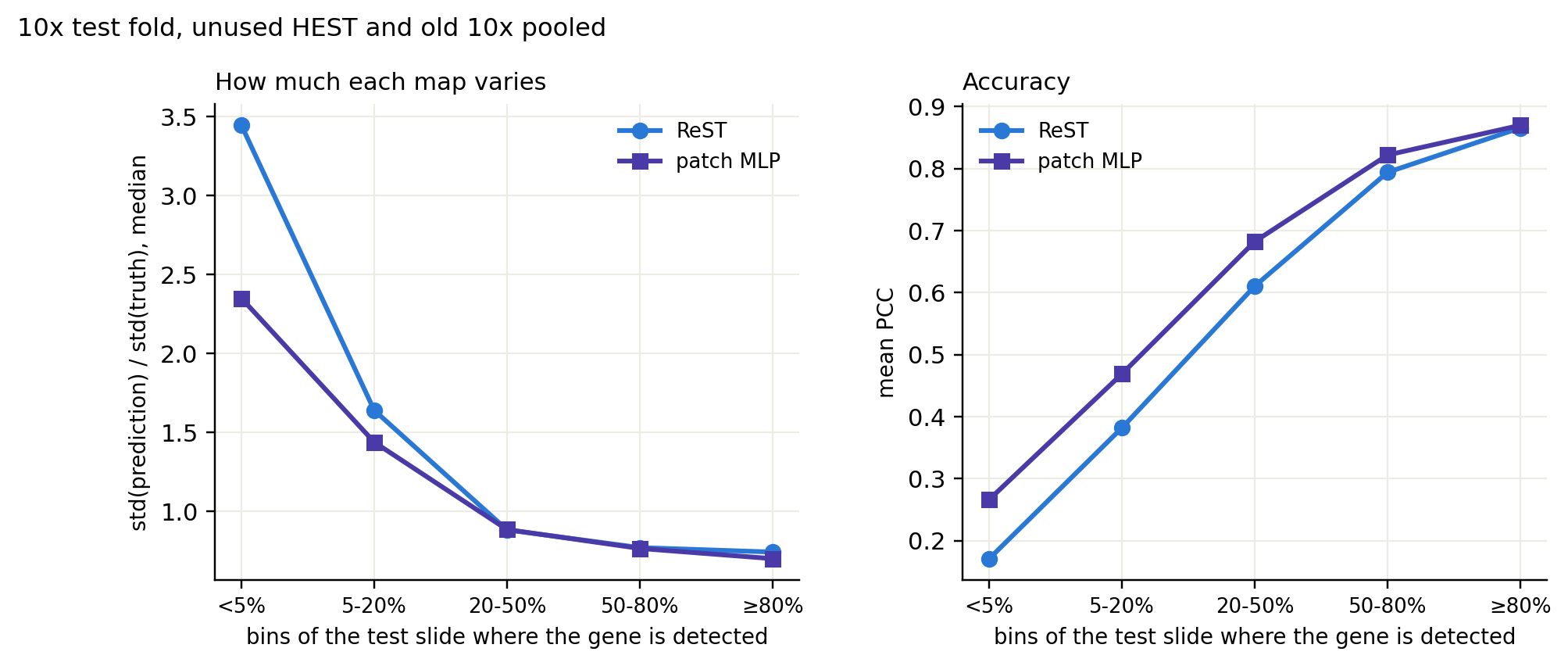
On genes detected in <5% of bins, ReST's maps vary 3.4× as much as the truth (MLP 2.3×) and the two models agree only at r = 0.48: ReST adds structure that is not there, it does not predict flat maps
Gene by gene the gap is noisy: detection and coverage together explain 6–7% of its variance
MLP gap: what fixes it
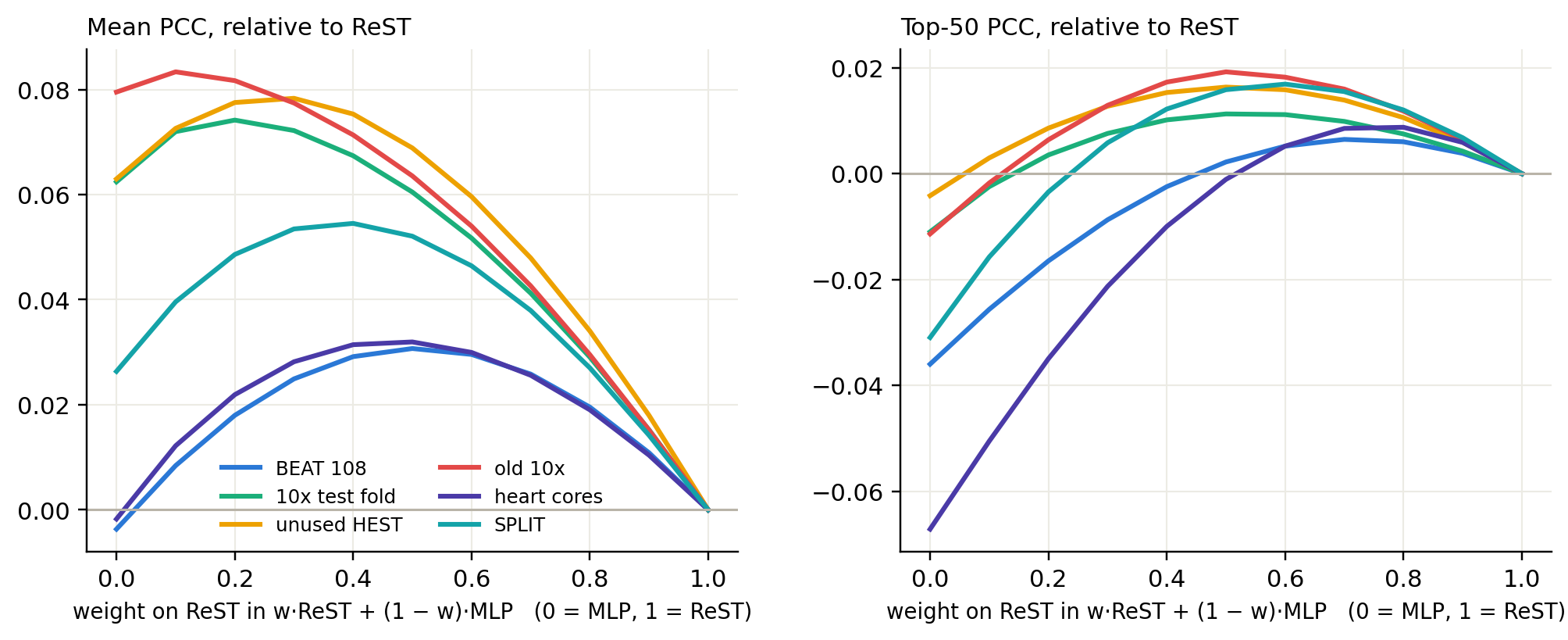
Averaging ReST with the MLP beats both models; the training-side fix to try first is a per-gene PCC loss
w·ReST + (1 − w)·MLP, change against ReST alone. Averaging is done on the predicted log1p maps, per bin.
mean PCC
top-50 PCC
setup
ReST
patch MLP
ReST + ReST ep63
ReST + MLP
ReST
patch MLP
ReST + ReST ep63
ReST + MLP
BEAT 108
0.608
0.604
0.616
0.638
0.872
0.836
0.870
0.874
10x test fold
0.548
0.611
0.573
0.609
0.874
0.863
0.867
0.885
unused HEST
0.576
0.639
0.596
0.644
0.886
0.882
0.878
0.903
old 10x
0.342
0.422
0.373
0.406
0.729
0.718
0.743
0.748
heart cores
0.239
0.237
0.234
0.271
0.668
0.601
0.649
0.667
ReST + ReST ep63: the same 50/50 average with a second, weaker ReST checkpoint (union ep63) in place of the MLP, as a control for plain averaging. Green: best per row and metric.
now, no retraining
Average ReST and the MLP 50/50. It beats both models on mean PCC on BEAT, unused HEST, heart cores and SPLIT, and matches or beats ReST's top-50 everywhere (heart cores: −0.001). Averaging with a second ReST gains much less, so the MLP adds something ReST lacks.
next, in training
Per-gene PCC loss. MSE weights each gene by its variance, so sparse genes barely count. The trainer already has a per-slide, per-gene PCC term (pcc_loss_weight); it was 0 for fov112. Done: with a rare-gene PCC term, this is the deck’s ReST.
Per-gene standardised MSE (targets z-scored with training means and stds): the same reweighting, keeping MSE.
Per-bin skip path: ReST predicts a correction on top of a per-bin MLP readout of the bin's own embedding, so context can only add.
Rare genes: sample training slides in proportion to how rarely their genes are measured.
ReST's failure 1: rarely trained genes
The fewer training slides measure a gene, the further ReST falls behind the patch MLP; the fixes close about 40% of that gap
Mean gene PCC (smoothed truth) per gene-slide, binned by how many of the 68 training slides measure the gene. ReST = the deck model (ep49 + 1 epoch per-gene PCC loss and coverage-weighted PCC, depth 4); ReST ep29 = MSE only. Heart cores and BEAT left out (BEAT has no rare genes; heart cores are tiny biopsies with uniformly low PCC).
0.36 → 0.40
ReST on genes measured on 1–2 training slides (8% of gene-slides); MLP 0.44
-0.085 → -0.044
gap to the MLP on those genes
Why: ReST takes one whole slide per step, so a gene on 2 of 68 slides is in ~3% of its steps; the MLP sees every bin of those slides. MSE also weights genes by their variance
What helped: the per-gene PCC loss (most of the gain) and up-weighting genes by 1/√(training slides)
Still open: 0.04 behind the MLP; on genes seen on 41+ slides ReST now leads (0.566 vs 0.556)
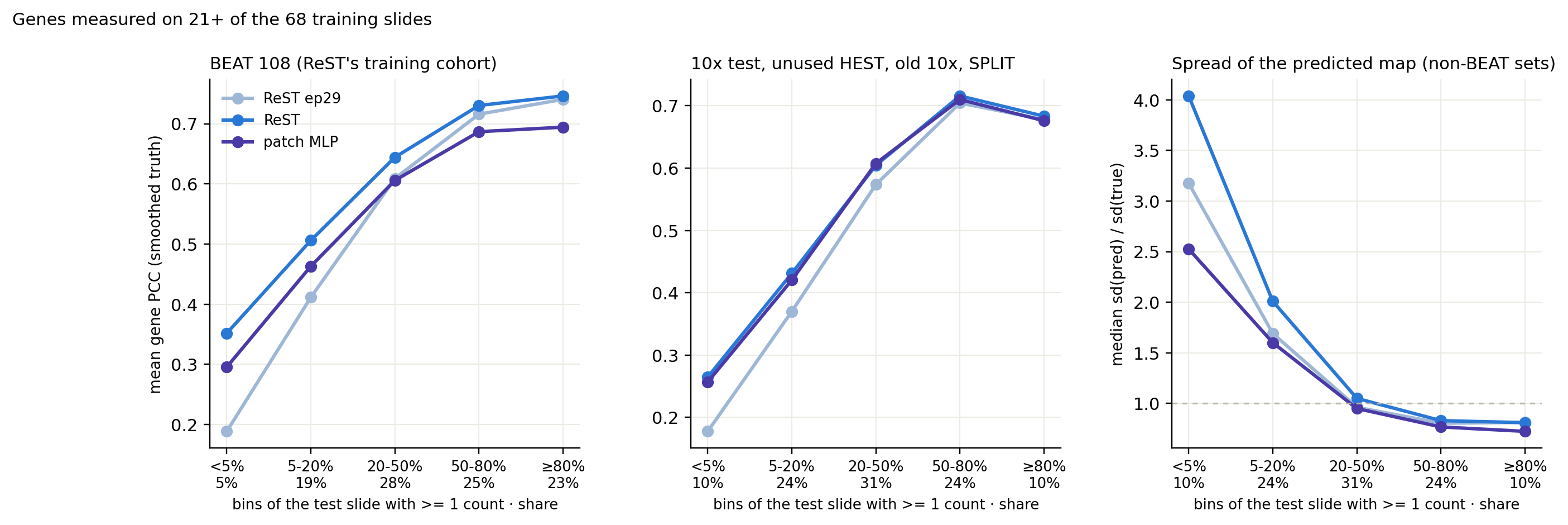
ReST's failure 2: low-count genes, even when well trained
Genes with a fraction of a count per bin: ReST over-predicts their structure; the PCC loss lifts accuracy but not the spread
Genes measured on 21+ training slides, binned by the share of the test slide's bins with at least one count (median counts per bin in those bins: <5% 0.04, 5-20% 0.17, 20-50% 0.87, 50-80% 3.78, ≥80% 14.22). Right: median spread of the predicted map relative to the truth's (dashed line = same spread).
the failure
On genes detected in <5% of bins, ReST ep29 scores 0.18 outside BEAT (MLP 0.26) and its maps vary 3.2× as much as the truth (MLP 2.5×): it paints structure that is not there
what the fix did
PCC on those genes: BEAT 0.19 → 0.35 (MLP 0.30); other sets 0.18 → 0.26 (MLP 0.26). From <5% detection on, ReST matches or beats the MLP
not fixed
The spread gets worse (4.0×): the PCC loss ignores scale. The slide-level distribution losses did not bring it down outside BEAT
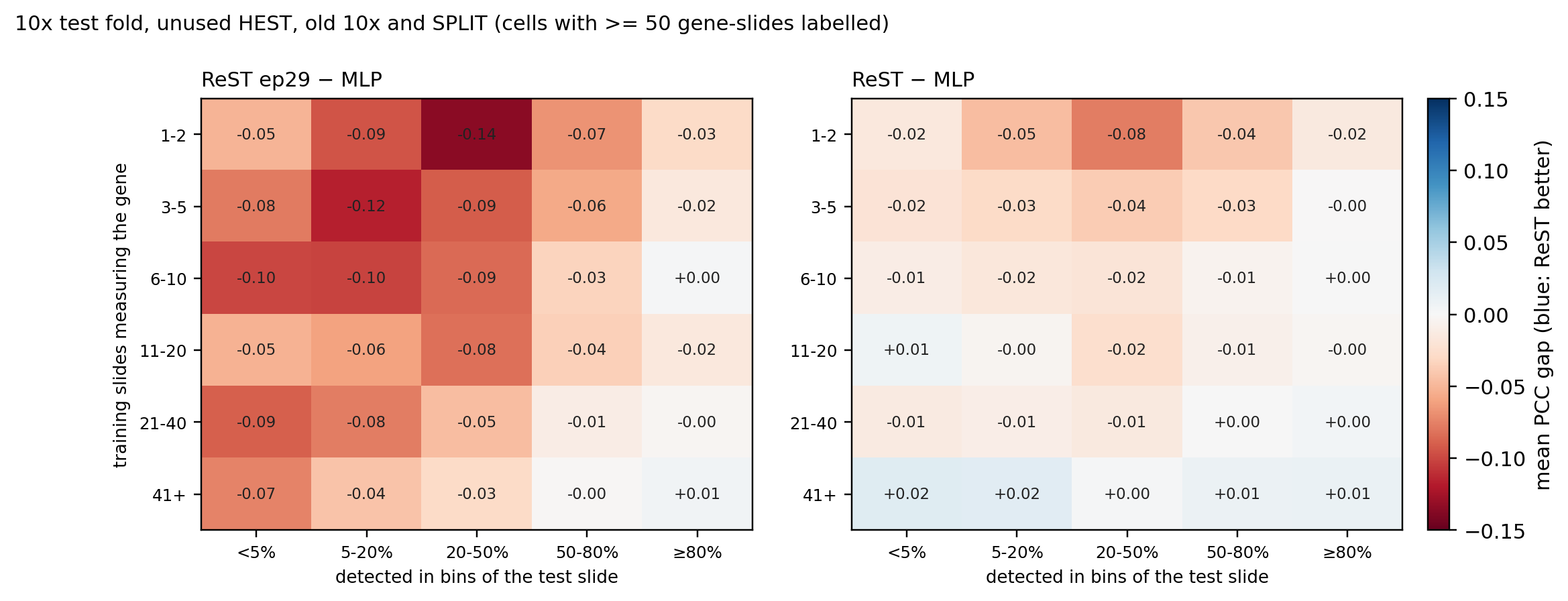
Where the remaining gap sits
After the fixes, the gap to the MLP sits mostly in genes that are both rarely trained and rarely detected
Mean PCC gap to the patch MLP per gene-slide, by training coverage (rows) and detection on the test slide (columns), on the sets ReST never trained on. Left: ReST ep29. Right: ReST (PCC + rare-gene fine-tune).
ReST ep29 trails the MLP in 28 of 30 cells (down to −0.14)
ReST trails in 21 of 30; largest gaps: −0.08 (1-2 slides, 20-50% detected); −0.05 (1-2 slides, 5-20% detected); −0.04 (1-2 slides, 50-80% detected)
Genes on 41+ training slides: +0.00 to +0.02
Tried and not worth it: slide-level distribution losses (−0.02 to −0.03 PCC, fidelity better on BEAT only); per-gene halting (the halt never fires)
Next: more coverage of rare genes (SPLIT + BEAT sections in training)
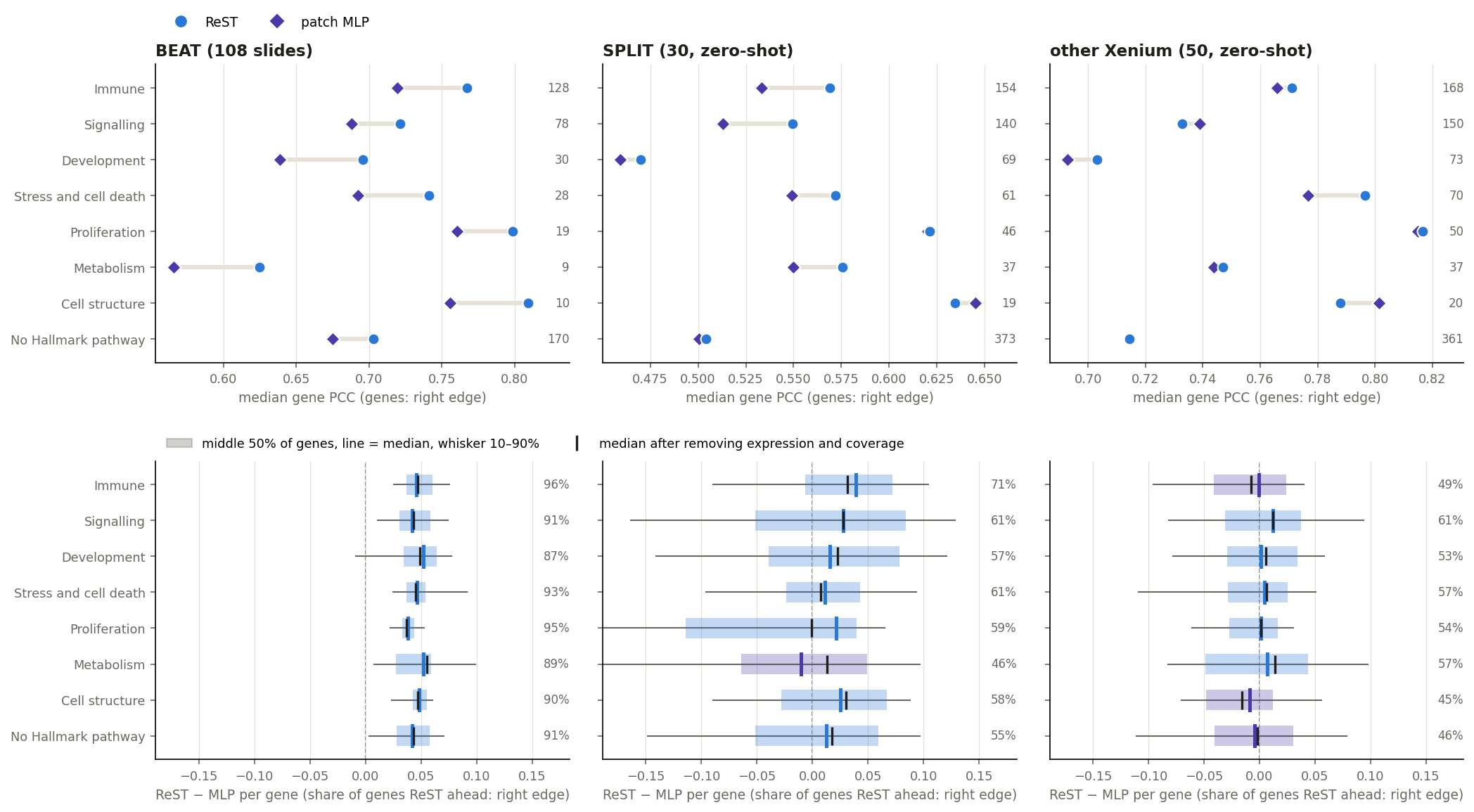
ReST vs MLP by gene category
ReST vs patch MLP per gene category, on BEAT and the two zero-shot cohorts
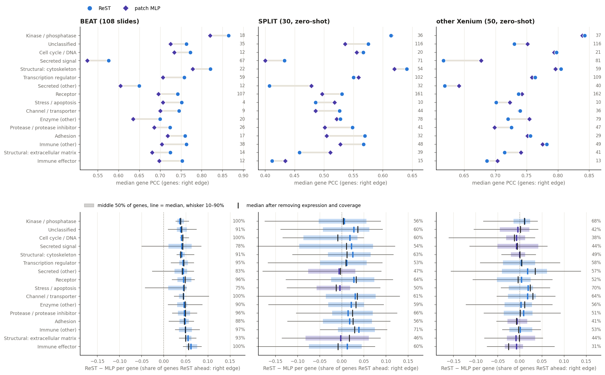
Top: median gene PCC per category (genes at the right edge). Bottom: per-gene ReST − MLP; black tick = the median after removing what expression level, detection and training coverage explain. Genes: measured and expressed (mean log1p ≥ 0.15) on ≥ 2 slides of the cohort; smoothed truth.
As the Hallmark view, with genes grouped by the protein class from their UniProt keywords (rules in the workbook).
reading
BEAT: ReST ahead in 16 of 16 protein classes (median per gene up to +0.061); only “secreted (other)” is level (+0.044)
Zero-shot, the MLP leads most on extracellular, sparse genes: secreted signals (+0.022 SPLIT, −0.008 other Xenium) and ECM (−0.003 SPLIT); secreted signals are detected in a median 32% of bins vs 46% for cytoskeleton genes
Sparsity explains part of it: after removing expression and coverage, secreted signals on other Xenium go to −0.006; ECM (+0.017) and immune effectors (−0.009) on SPLIT stay behind
Hallmark categories: within a zero-shot cohort the category medians span only −0.010 to +0.039 (SPLIT) and −0.009 to +0.012 (other Xenium): the cohort matters more than the category
Categories for review: deliverables/beat_gene_categories.xlsx (Hallmark category, UniProt class and keywords per gene; a corrected_category column this slide picks up on rebuild).
Video: how a pathway is scored
Play / pause: click the video or the space bar while it is focused · speed and full screen: the player menu
Video: how a niche is scored
Play / pause: click the video or the space bar while it is focused · speed and full screen: the player menu
The external model: DeepSpot-M
comparison with DeepSpot-M
external
DeepSpot-M
Public checkpoint, one tile at a time. Trained on ~500 Visium samples (15 datasets, 14 cancers); used zero-shot on every set.
Gene embeddings: the mean of its five sources (evo2, orthrus, ProtT5, scGPT, Apertus); the model card's example uses scGPT alone, and evo2 alone collapses to one shared map.
— Nonchev et al., medRxiv 2026
same inputs
Both models see the same 112 µm tile per bin (224 px at 0.5 µm/px, DeepSpot-M's native input) and are scored on the same bins, genes and truth.
ReST vs patch MLP vs DeepSpot-M on every test setup
comparison with DeepSpot-M
set
PCC
PCC top-50
Spearman
MLP > ReST slides, PCC
ReST
MLP
DS-M
ReST
MLP
DS-M
ReST
MLP
DS-M
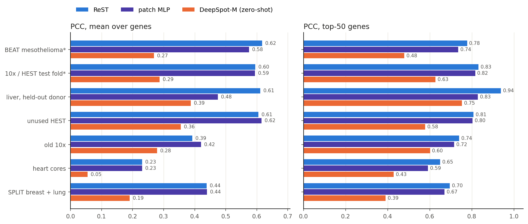
BEAT mesothelioma* (108 slides, 118 genes)
0.617
0.575
0.269
0.778
0.735
0.479
0.579
0.527
0.237
61 / 108
10x / HEST test fold* (18 slides, 372 genes)
0.595
0.594
0.287
0.832
0.817
0.627
0.591
0.581
0.291
17 / 18
liver, held-out donor (1 slides, 372 genes)
0.612
0.475
0.387
0.939
0.829
0.753
0.560
0.484
0.422
0 / 1
unused HEST, never seen (29 slides, 101 genes)
0.606
0.615
0.355
0.808
0.804
0.578
0.638
0.639
0.409
29 / 29
old 10x, never seen (3 slides, 231 genes)
0.393
0.421
0.279
0.741
0.716
0.602
0.391
0.424
0.282
3 / 3
heart biopsy cores, never seen (195 slides, 370 genes)
0.231
0.231
0.055
0.650
0.592
0.429
0.220
0.214
0.050
101 / 195
SPLIT breast + lung, never seen (30 slides, 129 genes)
0.438
0.439
0.191
0.696
0.671
0.390
0.414
0.409
0.182
24 / 30
set
PCC
PCC top-50
Spearman
MLP > ReST slides, PCC
ReST
MLP
DS-M
ReST
MLP
DS-M
ReST
MLP
DS-M
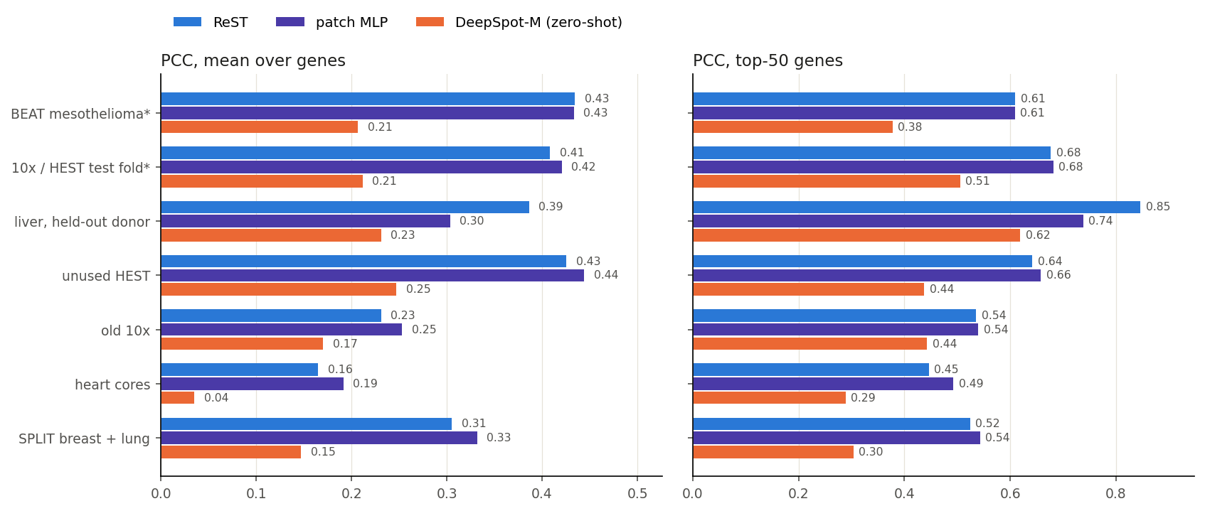
BEAT mesothelioma* (108 slides, 118 genes)
0.434
0.433
0.207
0.610
0.609
0.378
0.389
0.381
0.180
91 / 108
10x / HEST test fold* (18 slides, 372 genes)
0.408
0.421
0.212
0.677
0.681
0.505
0.383
0.390
0.206
18 / 18
liver, held-out donor (1 slides, 372 genes)
0.386
0.303
0.231
0.846
0.738
0.619
0.332
0.290
0.241
0 / 1
unused HEST, never seen (29 slides, 101 genes)
0.426
0.444
0.247
0.642
0.658
0.438
0.418
0.432
0.263
29 / 29
old 10x, never seen (3 slides, 231 genes)
0.231
0.253
0.170
0.536
0.540
0.443
0.217
0.240
0.162
3 / 3
heart biopsy cores, never seen (195 slides, 370 genes)
0.165
0.192
0.035
0.446
0.492
0.289
0.160
0.181
0.032
147 / 195
SPLIT breast + lung, never seen (30 slides, 129 genes)
0.306
0.332
0.147
0.524
0.543
0.304
0.281
0.302
0.138
28 / 30
set
partial PCC
partial Spearman
MLP > ReST slides, partial PCC
ReST
MLP
DS-M
ReST
MLP
DS-M
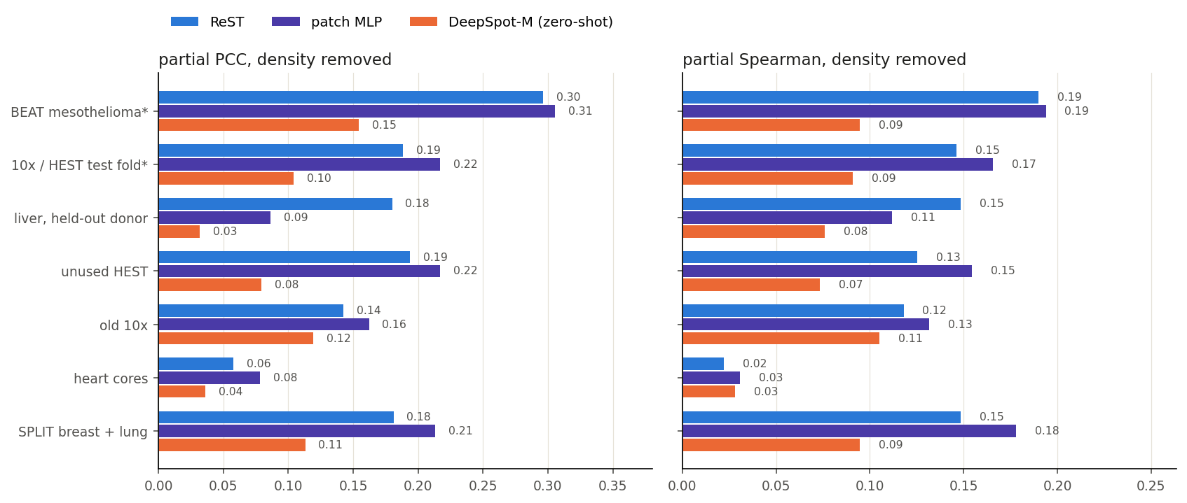
BEAT mesothelioma* (108 slides, 118 genes)
0.296
0.305
0.154
0.190
0.194
0.095
97 / 108
10x / HEST test fold* (18 slides, 372 genes)
0.188
0.217
0.104
0.146
0.166
0.091
16 / 18
liver, held-out donor (1 slides, 372 genes)
0.180
0.087
0.032
0.148
0.112
0.076
0 / 1
unused HEST, never seen (29 slides, 101 genes)
0.194
0.217
0.079
0.125
0.155
0.073
28 / 29
old 10x, never seen (3 slides, 231 genes)
0.143
0.162
0.119
0.118
0.132
0.105
3 / 3
heart biopsy cores, never seen (195 slides, 370 genes)
0.058
0.078
0.036
0.022
0.031
0.028
149 / 195
SPLIT breast + lung, never seen (30 slides, 129 genes)
0.181
0.213
0.113
0.149
0.178
0.095
28 / 30
set
PCC
PCC top-50
Spearman
MLP > ReST slides, PCC
ReST
MLP
DS-M
ReST
MLP
DS-M
ReST
MLP
DS-M
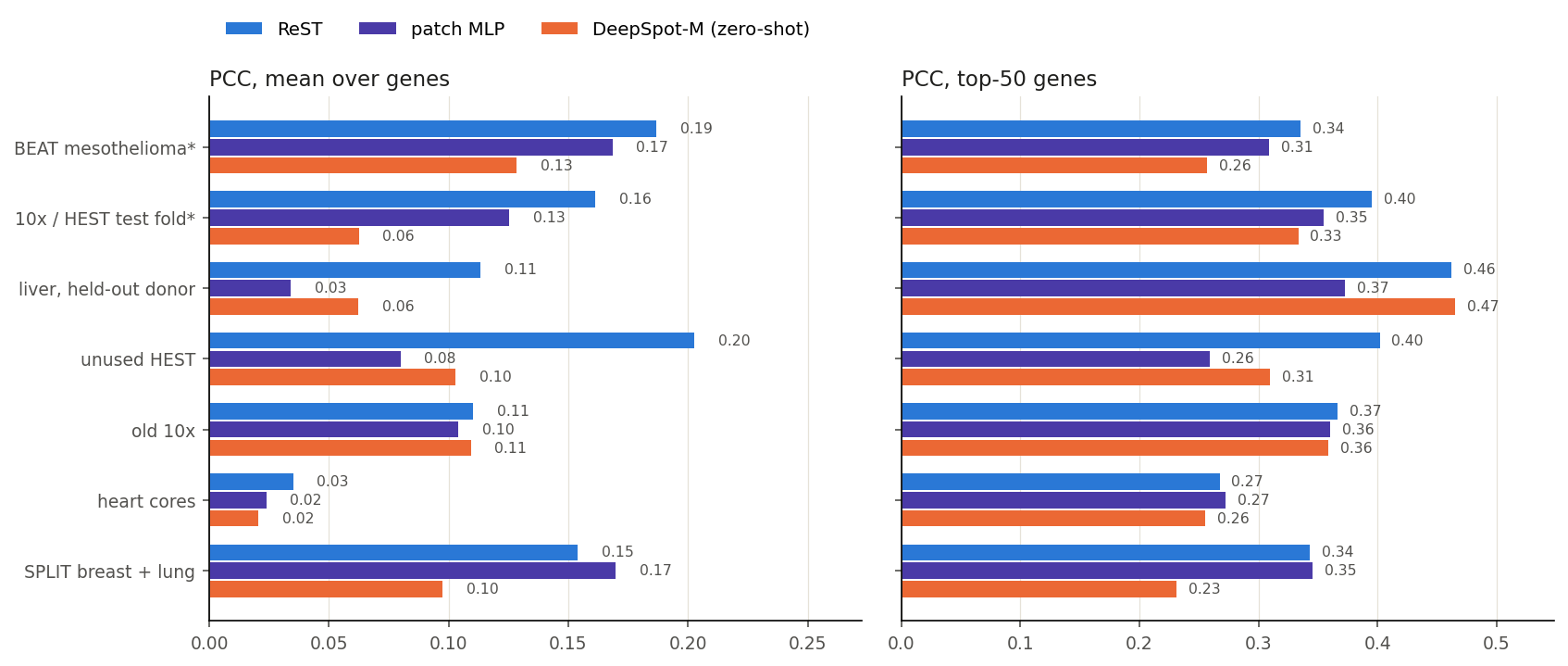
BEAT mesothelioma* (108 slides, 118 genes)
0.187
0.168
0.128
0.335
0.309
0.257
0.196
0.171
0.128
94 / 108
10x / HEST test fold* (18 slides, 372 genes)
0.161
0.125
0.062
0.395
0.355
0.333
0.150
0.112
0.061
14 / 18
liver, held-out donor (1 slides, 372 genes)
0.113
0.034
0.062
0.462
0.373
0.465
0.078
0.013
0.056
1 / 1
unused HEST, never seen (29 slides, 101 genes)
0.203
0.080
0.103
0.402
0.259
0.309
0.186
0.069
0.105
8 / 29
old 10x, never seen (3 slides, 231 genes)
0.110
0.104
0.109
0.367
0.360
0.359
0.105
0.101
0.108
3 / 3
heart biopsy cores, never seen (195 slides, 370 genes)
0.035
0.024
0.021
0.267
0.272
0.256
0.034
0.017
0.024
86 / 195
SPLIT breast + lung, never seen (30 slides, 129 genes)
0.154
0.170
0.097
0.343
0.345
0.231
0.165
0.176
0.102
28 / 30
Smoothed truth (each 55 µm bin with its 10 nearest; Phoenix also trains on k-NN-smoothed targets): mean over slides of the per-slide mean / top-50 over genes, on Phoenix’s fixed 1,000 bins per slide and the genes every model there predicts (genes per slide in brackets). green: best · * ReST and the MLP were trained on other patients / slides of these cohorts; DeepSpot-M is zero-shot. Density removed: each gene’s dependence on the bin’s log total taken out of prediction and truth.
BEAT, 108 held-out patients: ReST vs DeepSpot-M
comparison with DeepSpot-M
0.75 / 0.27
median gene PCC, ReST / DeepSpot-M
83% / 19%
gene–slide pairs with PCC ≥ 0.5
0.65 / 0.25
mean gene PCC per slide
108 / 108
slides where ReST is higher
Share of gene–slide pairs (expressed genes) at or above each PCC.
DeepSpot-M with evo2 gene embeddings only: median gene PCC 0.33. evo2 predicts nearly one shared map for all genes (80–90% of the variance on one component vs 30–57% measured), which raises per-gene PCC but removes most gene-specific signal.
BEAT examples: ReST vs DeepSpot-M
comparison with DeepSpot-M
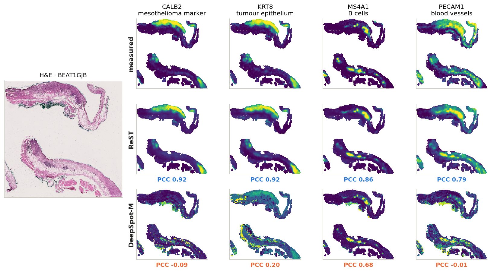
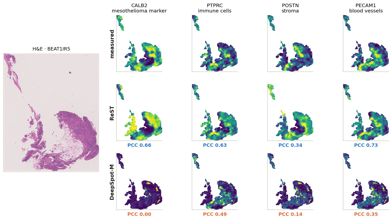
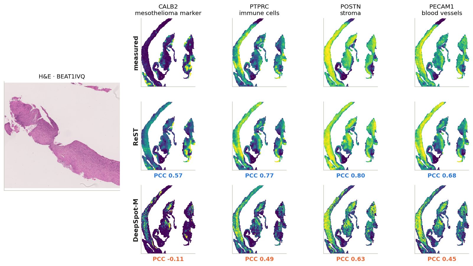
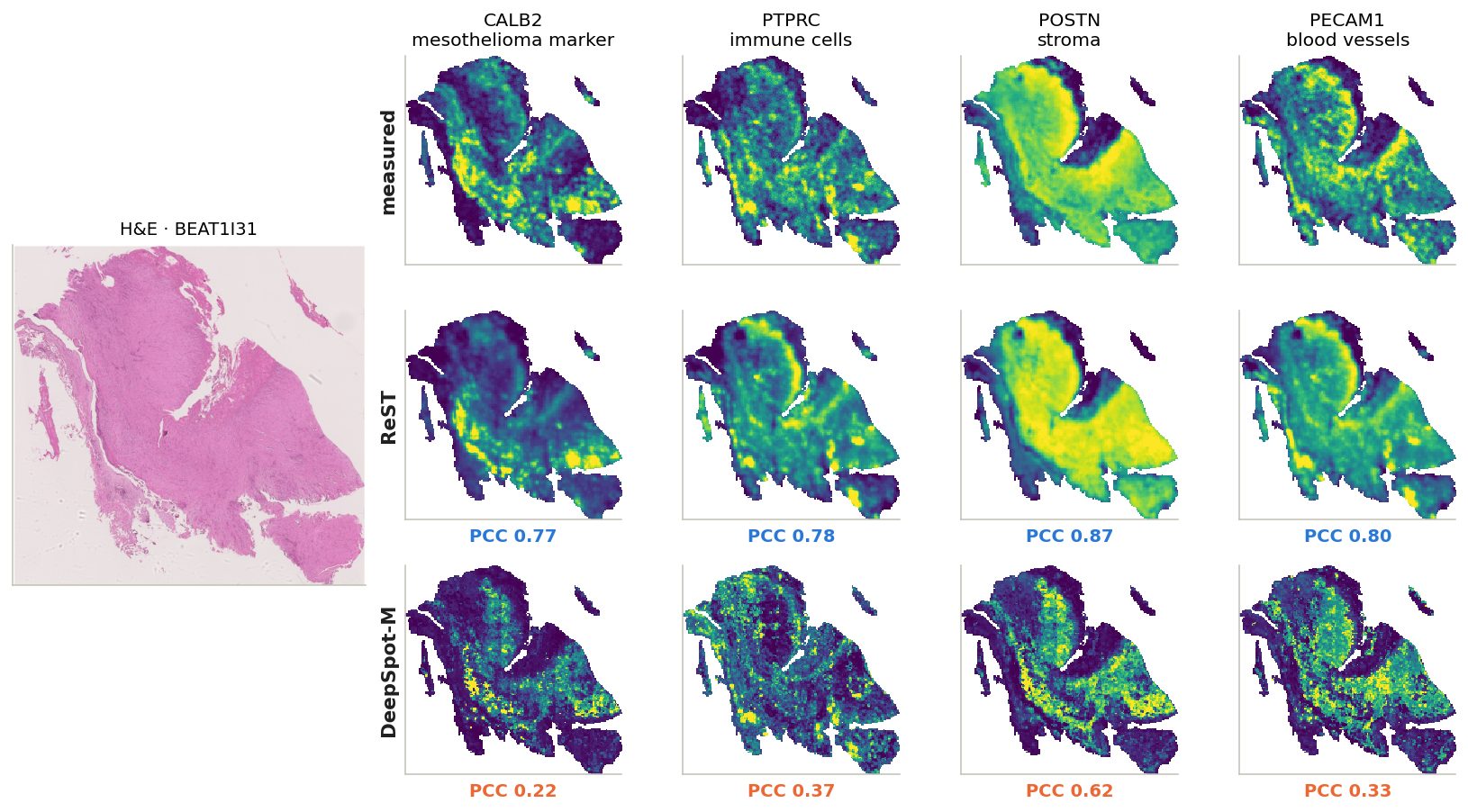
Six more slides spread over ReST's range (10th to 90th percentile of per-slide mean gene PCC); click a slide ID
BEAT1GJB: mean gene PCC over the slide, ReST 0.70, DeepSpot-M 0.22. Genes chosen for distinct patterns on this slide.
BEAT1IR5: mean gene PCC over the slide, ReST 0.50, DeepSpot-M 0.17. Same four genes on every example: tumour, immune, stroma, vessels.
BEAT1IVQ: mean gene PCC over the slide, ReST 0.58, DeepSpot-M 0.23. Same four genes on every example: tumour, immune, stroma, vessels.
BEAT1I31: mean gene PCC over the slide, ReST 0.67, DeepSpot-M 0.29. Same four genes on every example: tumour, immune, stroma, vessels.
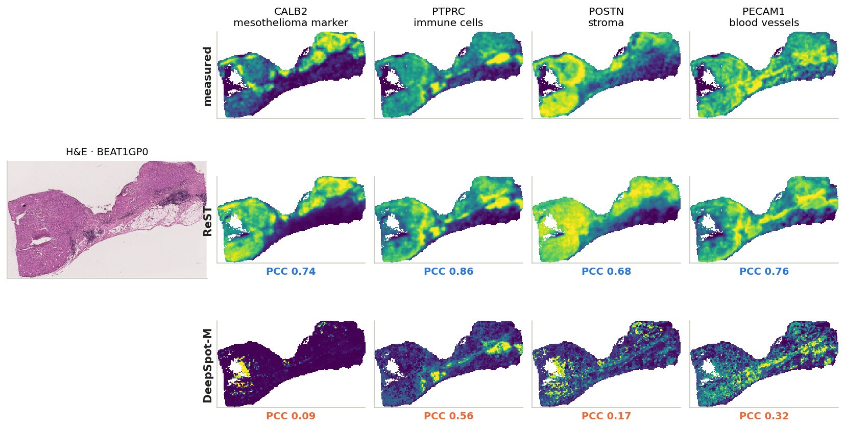
BEAT1GP0: mean gene PCC over the slide, ReST 0.71, DeepSpot-M 0.31. Same four genes on every example: tumour, immune, stroma, vessels.
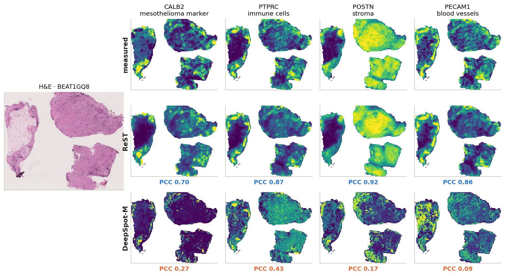
BEAT1GQ8: mean gene PCC over the slide, ReST 0.74, DeepSpot-M 0.24. Same four genes on every example: tumour, immune, stroma, vessels.
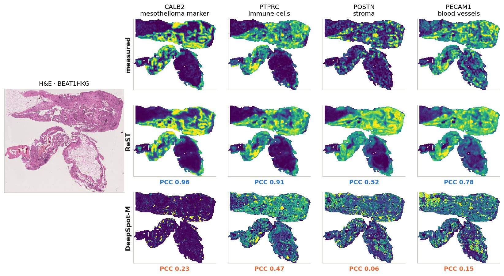
BEAT1HKG: mean gene PCC over the slide, ReST 0.77, DeepSpot-M 0.30. Same four genes on every example: tumour, immune, stroma, vessels.
10x Immuno-Oncology panel (380) + add-on (100): ReST vs DeepSpot-M
comparison with DeepSpot-M
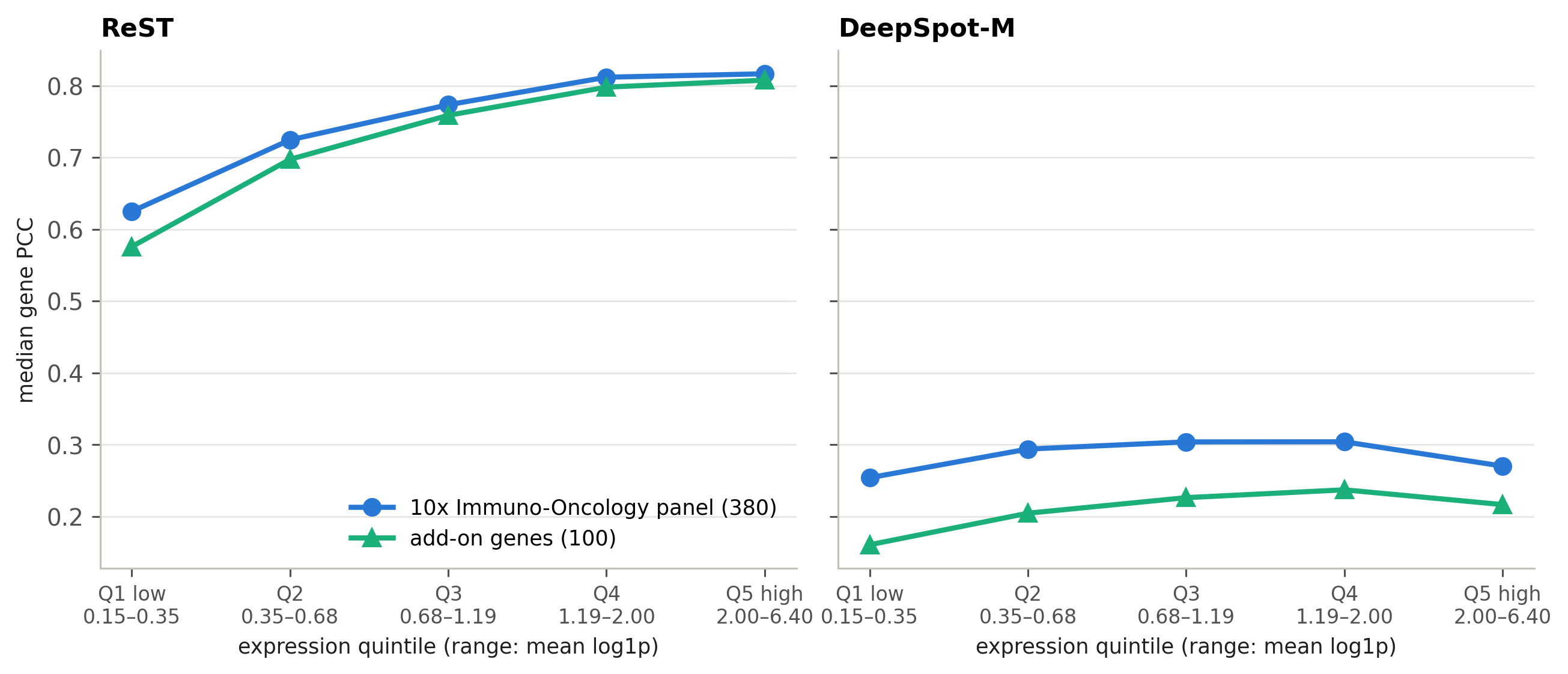
Median gene PCC within expression quintiles (defined below).
expressed genes
ReST
DeepSpot-M
10x panel
0.75
0.28
add-on
0.75
0.21
DeepSpot-M drops on the add-on genes; ReST does not.
expression quintiles
Every gene on every slide where it is expressed (mean log1p ≥ 0.15; 41,011 gene–slide pairs) is ranked by its mean expression on that slide and cut into 5 equal groups: Q1 = the lowest 20% … Q5 = the highest 20% (ranges under the axis).
Within each group: median PCC of the 10x-panel genes and of the add-on genes. Comparing inside a group removes the effect of expression level — add-on genes are more highly expressed, and PCC rises with expression.
PCC by cell type: ReST vs DeepSpot-M
comparison with DeepSpot-M
Left: marker-gene PCC. Right: profile agreement in dominated bins.
23 / 23
cell types whose markers ReST predicts better
Largest gap: malignant mesothelioma cell (0.79 vs 0.13).
Smallest: follicular dendritic cell (0.74 vs 0.59).
DeepSpot-M with evo2 gene embeddings only: ReST ep29 better on the markers of 23 of 23 cell types; median marker PCC 0.18. evo2 predicts nearly one shared map for all genes (80–90% of the variance on one component vs 30–57% measured), which raises per-gene PCC but removes most gene-specific signal.
Pathways: ReST vs DeepSpot-M
comparison with DeepSpot-M
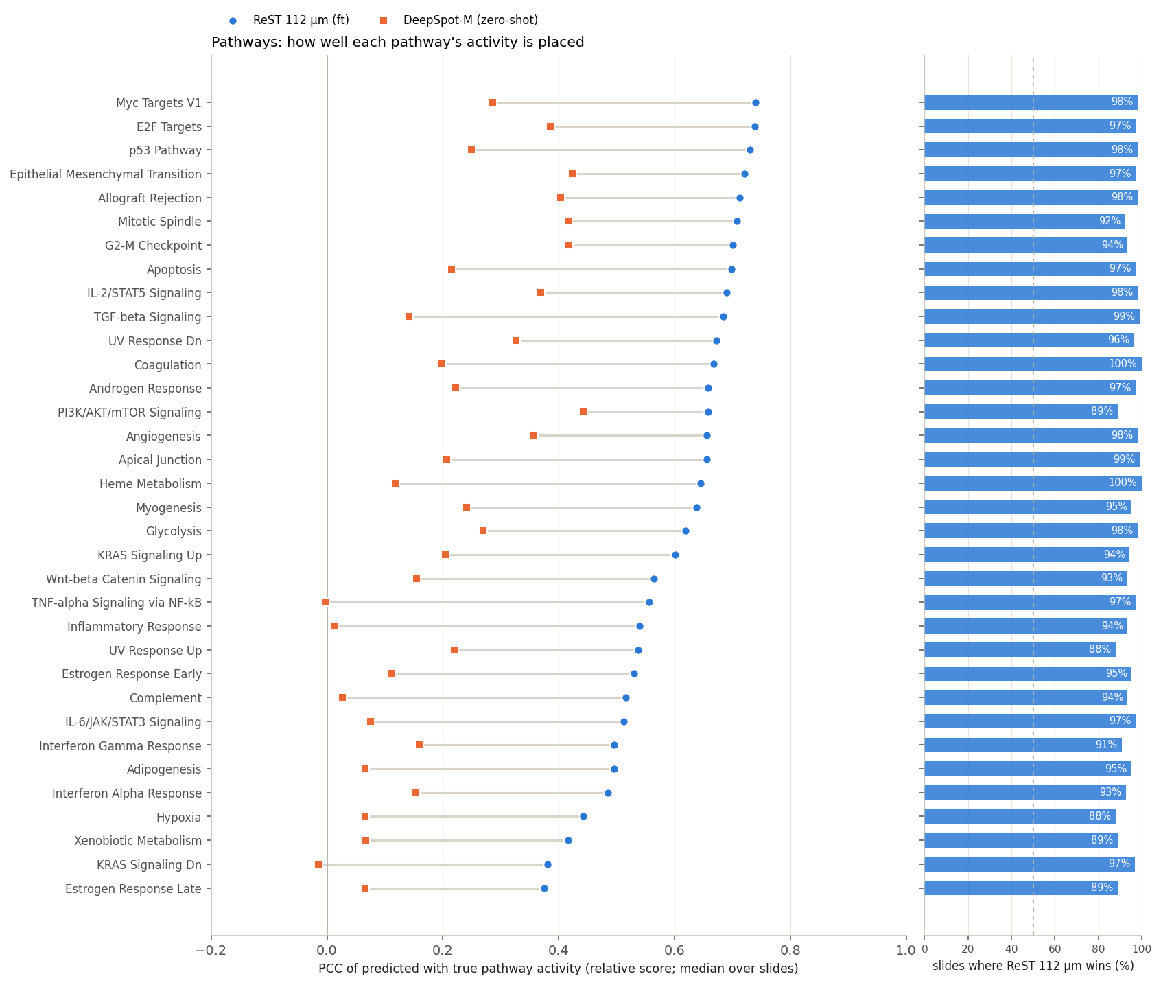
Median over slides of the relative-score PCC; right: share of slides on which ReST is higher.
34 / 34
pathways where ReST is higher
0.64 / 0.21
median pathway PCC, ReST / DeepSpot-M
DeepSpot-M with evo2 gene embeddings only: median pathway PCC 0.03. evo2 predicts nearly one shared map for all genes (80–90% of the variance on one component vs 30–57% measured), which raises per-gene PCC but removes most gene-specific signal.
Pathway regions: ReST vs DeepSpot-M
comparison with DeepSpot-M
Left: IoU (dashed: chance). Right: share of the predicted region where the truth is not active.
0.27 / 0.11
median IoU, ReST / DeepSpot-M
0.57 / 0.80
median spurious share (lower is better)
Pathway example: ReST vs DeepSpot-M
comparison with DeepSpot-M
Median over 108 slides: ReST 0.56, DeepSpot-M -0.00.
Niche similarity maps: ReST vs DeepSpot-M
comparison with DeepSpot-M
Click a niche
N6 · T cell + B cell: similarity to the niche's centroid from the truth, ReST and DeepSpot-M; AUROC on that slide under each map.
N12 · B cell + germinal center B cell: similarity to the niche's centroid from the truth, ReST and DeepSpot-M; AUROC on that slide under each map.
N11 · malignant mesothelioma cell: similarity to the niche's centroid from the truth, ReST and DeepSpot-M; AUROC on that slide under each map.
N15 · endothelial cell + pericyte: similarity to the niche's centroid from the truth, ReST and DeepSpot-M; AUROC on that slide under each map.
N3 · malignant mesothelioma cell: similarity to the niche's centroid from the truth, ReST and DeepSpot-M; AUROC on that slide under each map.
N19 · cycling T cell + CD8-positive, alpha-beta T cell: similarity to the niche's centroid from the truth, ReST and DeepSpot-M; AUROC on that slide under each map.
N4 · natural killer T cell + interferon response T cell: similarity to the niche's centroid from the truth, ReST and DeepSpot-M; AUROC on that slide under each map.
N10 · pericyte + macrophage: similarity to the niche's centroid from the truth, ReST and DeepSpot-M; AUROC on that slide under each map.
N9 · plasma cell: similarity to the niche's centroid from the truth, ReST and DeepSpot-M; AUROC on that slide under each map.
N0 · endothelial cell + fibroblast of lung: similarity to the niche's centroid from the truth, ReST and DeepSpot-M; AUROC on that slide under each map.
N2 · cycling fibroblast + fibroblast of lung: similarity to the niche's centroid from the truth, ReST and DeepSpot-M; AUROC on that slide under each map.
N18 · cycling fibroblast + fibroblast of lung: similarity to the niche's centroid from the truth, ReST and DeepSpot-M; AUROC on that slide under each map.
N16 · mesothelial cell + macrophage: similarity to the niche's centroid from the truth, ReST and DeepSpot-M; AUROC on that slide under each map.
N13 · cycling fibroblast + malignant mesothelioma cell: similarity to the niche's centroid from the truth, ReST and DeepSpot-M; AUROC on that slide under each map.
N8 · fibroblast of lung + cycling fibroblast: similarity to the niche's centroid from the truth, ReST and DeepSpot-M; AUROC on that slide under each map.
N17 · macrophage + cycling myeloid cell: similarity to the niche's centroid from the truth, ReST and DeepSpot-M; AUROC on that slide under each map.
N5 · malignant mesothelioma cell: similarity to the niche's centroid from the truth, ReST and DeepSpot-M; AUROC on that slide under each map.
N1 · cycling myeloid cell + interferon response myeloid cell: similarity to the niche's centroid from the truth, ReST and DeepSpot-M; AUROC on that slide under each map.
N14 · pericyte + endothelial cell: similarity to the niche's centroid from the truth, ReST and DeepSpot-M; AUROC on that slide under each map.
N7 · fibroblast of lung: similarity to the niche's centroid from the truth, ReST and DeepSpot-M; AUROC on that slide under each map.
Niches: ReST 88% vs DeepSpot-M 60%
comparison with DeepSpot-M
Median over slides; right: share of slides on which ReST is higher.
19 / 20
niches where ReST recovers more
Higher for DeepSpot-M: N12 B cell + germinal center B cell (99% vs 99%)
DeepSpot-M with evo2 gene embeddings only: median niche recovered 15%. evo2 predicts nearly one shared map for all genes (80–90% of the variance on one component vs 30–57% measured), which raises per-gene PCC but removes most gene-specific signal.
Niches and their cell types: ReST vs DeepSpot-M
comparison with DeepSpot-M
DeepSpot-M: niche signal recovered and its cell types' marker PCC (same layout as the ReST slide).
niche
signal recovered ReST · DS-M
cell-type PCC ReST · DS-M
N6 · T cell + B cell
100%
94%
0.68
0.34
N12 · B cell + germinal center B cell
99%
99%
0.73
0.55
N11 · malignant mesothelioma cell
96%
76%
0.79
0.13
N15 · endothelial cell + pericyte
95%
60%
0.65
0.22
N3 · malignant mesothelioma cell
93%
80%
0.79
0.13
N19 · cycling T cell + CD8-positive, alpha-beta T cell
93%
80%
0.68
0.18
N4 · natural killer T cell + interferon response T cell
Spearman r across the 20 niches (niche signal vs cell-type PCC; +1 same order, 0 unrelated): ReST +0.22, DeepSpot-M +0.46. DeepSpot-M's best-recovered niches: N12 B cell + germinal center B cell, N6 T cell + B cell. Same 108 slides.
Niche calls: ReST vs DeepSpot-M
comparison with DeepSpot-M
Same slides; DeepSpot-M column added: the same nearest-centroid call on its predicted expression.
Same slides; DeepSpot-M column added: the same nearest-centroid call on its predicted expression.
Same slides; DeepSpot-M column added: the same nearest-centroid call on its predicted expression.
Same slides; DeepSpot-M column added: the same nearest-centroid call on its predicted expression.
Same slides; DeepSpot-M column added: the same nearest-centroid call on its predicted expression.
Same slides; DeepSpot-M column added: the same nearest-centroid call on its predicted expression.
Same slides; DeepSpot-M column added: the same nearest-centroid call on its predicted expression.
Same slides; DeepSpot-M column added: the same nearest-centroid call on its predicted expression.
CellCharter niche
The reference. A bin takes the niche of ≥ 50% of its cells (CellCharter labels cells from their own and their neighbours' expression). Mixed bins: blank.
called from truth
Each bin's measured expression, assigned to the most similar niche centroid (PCC across genes). The reference, not a ceiling: ReST predicts all bins jointly, so its bins carry context and beat it on 11% of niche-slide pairs.
called from ReST
The same rule on ReST's predicted expression (z-scored per gene over the slide), with the same centroids from the measured data. Compare with the middle map, “called from truth”.
Percentages: bins whose call matches the CellCharter niche. Colours: the slide's 8 most common niches; grey: the rest.
Summary: ReST vs zero-shot DeepSpot-M
comparison with DeepSpot-M
1ReST is higher on every test setup and on 344 of 354 slides.
2BEAT: median gene PCC 0.75 vs 0.27; add-on minus 10x panel: ReST +0.00, DeepSpot-M -0.07.
3Markers of 23 of 23 cell types, 34 of 34 pathways (IoU 0.27 vs 0.11) and 19 of 20 niches (88% vs 60%) are predicted better by ReST.
DeepSpot-M saw none of these cohorts; ReST trained on other patients of BEAT and of the 10x collection.
← / → navigate
click: zoom in at that point · shift-click or −: zoom out · wheel: zoom · drag: pan · 0: fit · Esc: close